---

There are many different types of genres present in the music industry. However, the basic genres will have a few principle aspects that make it easier to identify them. Genres are used to tag and define different kinds of music based on the way they are composed or based on their musical form and musical style.

In this article, you’ll learn to build your own model which will take in a song as an input and predict or classify that particular song in one of the basic genres. We’ll be classifying among the following groups: blues, classical, country, disco, hiphop, jazz, metal, pop, reggae, and rock.

The model will be built using long short-term memory (LSTM) networks. Don’t worry if you don’t know what LSTM is. This article will give you a brief understanding of LSTM and its workings.

Our article will be divided into these segments:

1. Prerequisites
2. Theory
3. Data Preprocessing
4. Training the Model
5. Predicting on New Data

Prerequisites

There are a few prerequisites you’ll need to have before you start this project. The first thing you’ll need is the dataset. The music data which I’ve used for this project can be downloaded from Kaggle at https://www.kaggle.com/andradaolteanu/gtzan-dataset-music-genre-classification.

Note that this dataset contains 10 classes with 100 songs within each class. This might not seem like a lot for a machine learning project, so that’s why in the next section I’ll show you how to increase the number of training data for each class of genre.

There are a few modules which will be required for you to install on your PC/laptop in order to get started. We’ll be building the entire LSTM model using TensorFlow, coded in Python. We’ll be working with Python 3.6 or higher. (If you’re currently using Python 2.7, it’s required for you to use Python 3.6 or higher for full support and functionality.)

The following are the required Python packages to be installed:

1. TensorFlow: Machine learning software library.
2. Librosa: Speech processing library to extract features from songs.
3. NumPy: Mathematical model for scientific computing.
4. Scikit-learn (formerly scikits.learn and also known as sklearn): Another machine learning model (we’ll use this library to split training and testing data).
5. JSON: Used to “jsonify” the dataset (explained in the next section).
6. Pytdub: Converts mp3 to wav files.

These modules can be installed using PIP or Conda. You can find many online sources and YouTube videos on getting started with PIP or Conda.

Once the above modules are installed, let’s get coding!

Theory

For any machine learning project, there are two main things in it: feature extraction from the data; and training the model.

For audio and music feature extraction for machine learning purposes, usually mel-frequency cepstral coefficients (MFCCs) are extracted from the song or audio. These features are used to train the model.

MFCC feature extraction is a way to extract only relevant information from an audio.

To explain this better, when we represent an audio file in digital format, the computer looks at it as a wave with the X axis as time and the Y axis as amplitude. This is shown in Figure 1.

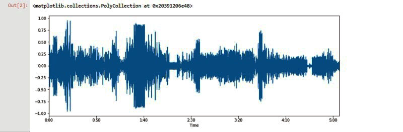
FIGURE 1. Music representation in amplitude and time.

---

This format of representation does not give us much information about the audio or song. Hence, we represent the audio in the frequency domain by using something called Fast Fourier Transform (FFT).

FFT is a mathematical algorithm that found its major use in signal processing, which is used to convert the time domain into the frequency domain. You can refer to https://www.nti-audio.com/en/support/know-how/fast-fourier-transform-fft#:~:text=Fast%20Fourier%20Transformation%20FFT%20%2D%20Basics,frequency%20information%20about%20the%20signal or watch a YouTube video on what FFT is and exactly how it works.

Using this FFT, we convert our input audio file and represent it in the frequency and time domain. The graph which displays the audio data in the frequency and time domains is called a spectogram, represented in Figure 2.

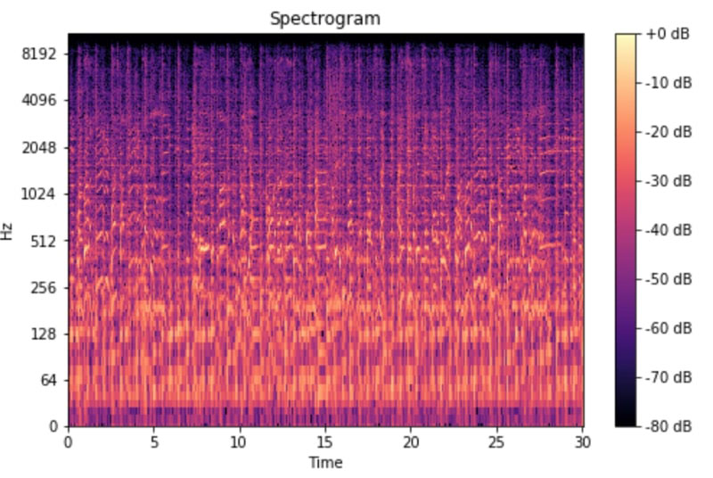
FIGURE 2. Spectogram.

---

A spectrogram is a bunch of FFTs stacked on top of each other. It’s a way to visually represent a signal’s loudness, or amplitude, as it varies over time at different frequencies. Here, the Y axis is converted to a log scale, and the color dimension is converted to decibels (you can think of this as the log scale of the amplitude). This is done as humans can only perceive a very small and concentrated range of frequencies and amplitudes. The human ear works on the principle of a logarithmic scale.

A normal spectogram can be used for extracting features, but this still contains some amount of additional information which is not required. As the human ear works on the logarithmic scale and not the linear scale, we use mel spectograms which convert this spectogram into a logarithmic representation to get the features more accurately by removing or eliminating unwanted features.

A mel spectrogram is a spectrogram where the frequencies are converted to the mel scale. Figure 3 shows the mel spectrogram.

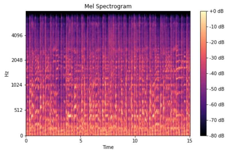
FIGURE 3. Mel spectogram.

---

Coming back to the main topic, the MFCCs uses a mel scale which is used to extract the features from an audio signal, which when represented as a graph, turns out to be a mel spectrogram. So, in a nutshell, what we see on a mel spectrogram is the exact features we need for training our model.

I have found this brilliant article which explains everything about MFCCs in depth at http://practicalcryptography.com/miscellaneous/machine-learning/guide-mel-frequency-cepstral-coefficients-mfccs.

Once we have our dataset ready, it’s time to train our model. Music is a time series data. That means, music is linear to time. LSTMs are pretty good at extracting patterns in input feature space, where the input data spans over long sequences. Given the gated architecture of LSTMs that have this ability to manipulate its memory state, they’re ideal for such problems.

For more information, you can refer to the blog at https://medium.com/@kangeugine/long-short-term-memory-lstm-concept-cb3283934359#:~:text=LSTM%20is%20a%20recurrent%20neural,time%20lags%20of%20unknown%20duration.&text=RNN%20cell%20takes%20in%20two,and%20observation%20at%20time%20%3D%20t.

Data Preprocessing

As mentioned, the data set which we are going to use here was downloaded from Kaggle and has about 100 songs under each of the 10 labels or genres. Each of the songs are 30 seconds long. Again, this amount of data is significantly less than usual for training an LSTM model.

To counter this problem, I split every audio file into 10 segments with each segment being three seconds long.

Hence, the number of songs under each label is now 1,000, which is a decent number to train the model to achieve good accuracy.

Now that we have our data ready, we need to extract the features which will be suitable to feed into our network. The feature extraction will be done by using MFCCs. Librosa is used to extract the features from each of the audio segments. We create a dictionary with the label or category of the genre as the key and all the extracted features from all the 1,000 segments as an array of features under that label.

Once we do this in a loop for all 10 categories, we dump the dictionary into a JSON file. This JSON file thus becomes our dataset on which the model will be trained.

Moving into the coding for dataset preprocessing, we first define the number of segments and sample rate of each segment. The sample rate is required to know the playback speed of the song. Here, we keep it constant for every segment:

dataset_path = “genres”
jsonpath = “data_json”
sample_rate = 22050
samples_per_track = sample_rate * 30
num_segment=10

We then create a loop in which we open up every song file from every genre folder and split it into 10 segments. We then extract the MFCC features for each segment and append it to the dictionary under the genre name (which is also the folder name).

Figure 4 shows the code snippet for the data processing function (this can be found at the github link listed in the Resources).

The script in Figure 4 will create segments, and extract features and dump the features into the data_json.json file.

FIGURE 4.

---

Training the Model

LSTM is used for training the model. Before we build the model, we have to load it into our program and split it into training and testing. This is done by opening the JSON file which we created in the last section and converting it into NumPy arrays for easy computation.

This method is shown in the snippet below:

def load_data(data_path):
    print(“Data loading\n”)
    with open(data_path, “r”) as fp:
        data = json.load(fp)
    x = np.array(data[“mfcc”])
    y = np.array(data[“labels”])
    print(“Loaded Data”)
    return x, y

After loading the data, we prepare the data and split it into train and test sets as mentioned earlier. This is done by using the following sklearn’s train_test_split function:

def prepare_datasets(test_size,val_size):
    #load the data
    x, y = load_data(data_path)
    x_train, x_test, y_train, y_test =  
    train_test_split(x,y,test_size = test_size)
    x_train, x_val, y_train, y_val =
    train_test_split(x_train,y_train,test_size = val_size)
    return x_train, x_val, x_test, y_train, y_val, y_test

Next, the LSTM network is created using TensorFlow. Here, we have created an LSTM network of four layers, including two hidden layers. The following code snippet shows the network creation:

def build_model(input_shape):
    model = tf.keras.Sequential()
    model.add(tf.keras.layers.LSTM(64, input_shape = input_shape)
    model.add(tf.keras.layers.LSTM(64))
    model.add(tf.keras.layers.Dense(64, activation=”relu”))
    model.add(tf.keras.layers.Dense(10,activation = “softmax”))
    return model

We initialize the model as sequential and add one input layer with 64 as the number of neurons in that layer, one hidden layer, one dense LSTM layer, and an output layer with 10 neurons for the 10 genres. The size of the input layer depends on the size of the MFCC coefficient which we are passing as an argument input_shape. You can experiment with more hidden layers and test the accuracy.

Once all the methods and functions have been defined, it’s time to call them and train our classification model:

if __name__ == “__main__”:
    x_train, x_val, x_test, y_train, y_val, y_test =     
    prepare_datasets(0.25, 0.2)
    input_shape = (x_train.shape[1],x_train.shape[2])
    model = build_model(input_shape)
    # compile model
    optimiser = tf.keras.optimizers.Adam(lr=0.001)
    model.compile(optimizer=optimiser,
                  loss=’sparse_categorical_crossentropy’,
                  metrics=[‘accuracy’])
    model.summary()
    model.fit(x_train, y_train, validation_data=(x_val, y_val),
                                     batch_size=32, epochs=50)
    model.save(“model_RNN_LSTM.h5”)
    print(“Saved model to disk”)

First, we call the prepare_datasets function and pass the test date percentage and validation data percentage. Validation data is some part of the training data, with which the model is not trained and is used to validate the model. The validation set tells us whether the data is performing well or not after the training is done. Next, we call the build_model function to build the LSTM network and compile it. Compiling is used to add the optimizer (which defines the learning rate) and the loss calculating function.

Here, we have used the categorical crossentropy mathematical function. You can read more about this at https://gombru.github.io/2018/05/23/cross_entropy_loss/#:~:text=TensorFlow%3A%20log_loss.-,Categorical%20Cross%2DEntropy%20loss,used%20for%20multi%2Dclass%20classification.

After compiling, model.fit() is used to train the model on our data. The training can take about 1-1.5 hours depending on your hardware.

We don’t want to keep training our model in order to test it. So, after training, we save the model so we can use this saved file to predict on our new data. At the end of the training, you can see the accuracy achieved.

Testing and Predicting

Congratulations! Our model has been trained! Now it’s time to check how well it predicts different songs and classifies it into different genres.

Before we start with the testing and prediction of new songs, we must define the constants:

###########################################################################
just_path = “genres/blues/”
song_path = “genres/blues/1.wav”
song_name = “1”
##########################################################################
#Constants which depend on the model. If you train the model with different values,
#need to change those values here too
num_mfcc = 13
n_fft=2048
hop_length = 512
sample_rate = 22050
samples_per_track = sample_rate * 30
num_segment = 10
###########################################################################

If you remember, we had trained our model with songs 30 seconds long, so the model will accept song segments of 30 seconds at a time. For this, we split the input song to be predicted into multiple segments of 30 seconds long.

There are three different scenarios for this: Song length is less than 30 seconds; song length equals 30 seconds; or song length is greater than 30 seconds.

For a song length less than 30 seconds, we show an error message because the minimum is not achieved. For a song length greater than 30 seconds, we split the entire song into multiple segments of 30 seconds each and feed each segment into the model.

The following snippet is for the above-mentioned scenarios:

#load the song
x, sr = librosa.load(song_path, sr = sample_rate)
song_length = int(librosa.get_duration(filename=song_path))
flag = 0
if song_length > 30:
        print(“Song is greater than 30 seconds”)
        samples_per_track_30 = sample_rate * song_length
        parts = int(song_length/30)
        samples_per_segment_30 = int(samples_per_track_30 / (parts))
        flag = 1
        print(“Song sliced into “+str(parts)+” parts”)
elif song_length == 30:
        parts = 1
        flag = 0
else:
        print(“Too short, enter a song of length minimum 30
        seconds”)
        flag = 2
for i in range(0,parts):
        if flag == 1:
            print(“Song snippet “,i+1)
            start30 = samples_per_segment_30 * i
            finish30 = start30 + samples_per_segment_30
            y = x[start30:finish30]
            #print(len(y))
elif flag == 0:
            print(“Song is 30 seconds, no slicing”)

Next, we load the saved model and define the different classes or genres. The model will predict a number from 0 to 9, and each number will represent a genre as defined during training:

model = tf.keras.models.load_model(“model_RNN_LSTM.h5”)
   
classes = [“Blues”,”Classical”,”Country”,”Disco”,”Hiphop”,
                “Jazz”,”Metal”,”Pop”,”Reggae”,”Rock”]

The model predicts a genre for each and every segment of the input song. The most predicted genres combine all the predictions of all the sliced segments of a particular input song and gives the final prediction.

For example, if a song length 120 seconds is given as input, it’s first split into three segments of 30 seconds each and each segment is given as input to the model which predicts a particular genre. The genre which is predicted the most number of times on average is the genre of the entire song.

For prediction, we again extract the MFCC features of each segment and then call model.predict() to get a prediction:

for n in range(num_segment):
            start = samples_per_segment * n
            finish = start + samples_per_segment
            #print(len(y[start:finish]))
            mfcc = librosa.feature.mfcc(y[start:finish],
            sample_rate, n_mfcc = num_mfcc, n_fft = n_fft,   
            hop_length = hop_length)
            mfcc = mfcc.T
            mfcc = mfcc.reshape(1, mfcc.shape[0], mfcc.shape[1])
         
            array = model.predict(mfcc)*100
            array = array.tolist()
#find maximum percentage class predicted
class_predictions.append(array[0].index(max(array[0])))
occurence_dict = {}
for i in class_predictions:
            if i not in occurence_dict:
                occurence_dict[i] = 1
            else:
                occurence_dict[i] +=1
max_key = max(occurence_dict, key=occurence_dict.get)
        prediction_per_part.append(classes[max_key])

prediction = max(set(prediction_per_part), key = prediction_per_part.count)
print(prediction)

Now you know how Spotify classifies your music for you!  SV

---

---