---

Large scale neural networks using sophisticated libraries can be burdensome for small projects. So, an alternative neural network you can program in a few lines of conventional code will be explained. The processor and memory requirements are quite low and suited to low cost single-board computers (SBCs). While still an experimental algorithm, it can produce complex and interesting behaviors for your robotics projects.

The Basics

Artificial neural networks are comprised of multiple layers. Each layer has two basic components:

• An adjustable system of weighted sums.
• A single fixed (nonadjustable) activation function, reused for each weighted sum.

The ReLU activation function in Figure 1 is a very popular choice.

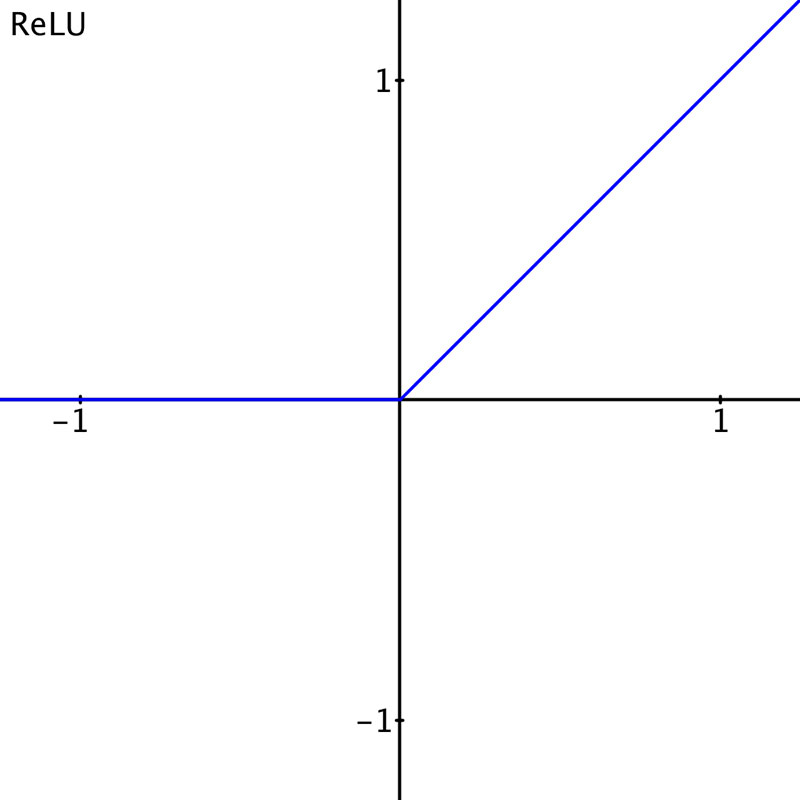
Figure 1. The ReLU activation function. For all inputs below zero, the output is zero. For all inputs above zero, the response is 1-to-1. An input of 0.5 gives an output of 0.5, and an input of 1 gives an output of 1 which results in a 45 degree slope in the graph. It’s the same response as a closed switch.

---

It outputs zero for inputs less than zero. For inputs greater than zero, it just copies the input to the output. Figure 2 shows a ReLU neural network layer with inputs a, b, c, and d.

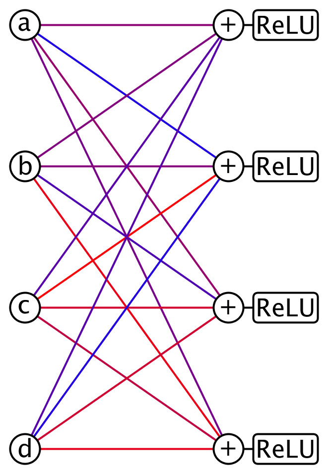
Figure 2. A ReLU neural network layer. Several of these layers composed together give a deep neural network. The values a, b, c, and d are multiplied by edge weights before summation. For example, blue could be –10 and red +10 and intermediate colors have an intermediate value between –10 and +10.

---

The network is expensive to compute because there are so many weighted sums to calculate. In Figure 2, the width of the layer is only four, yet already 16 multiply and 16 add operations are needed. As the width increases, the situation only gets worse. If n is the width of the network, then n squared multiplies and n squared add operations are required, contributing the bulk of the computational cost of the layer.

Fast Transforms

For lightweight robotics applications, it would be better to reduce the calculation cost of the weighted sums. One approach is to make use of simple transforms that involve patterns of addition and subtraction. One such device is the fast Walsh Hadamard transform (WHT).

Given an array of two elements a, b:

WHT(a, b) = a+b, a-b

For an array of four elements (a,b,c,d), obtain the two-point transforms of a,b and c,d and then add and subtract the alike (in pattern of add and subtract) terms:

WHT(a, b) = a+b, a-b
WHT(c, d) = c+d, c-d

The alike terms are a+b, c+d, and also a-b, c-d. Adding and subtracting those gives:

WHT(a, b, c, d) = a+b+c+d, a+b-c-d, a-b+c-d, a-b-c+d

You know to stop because there are no more alike terms to add and subtract. Transforms of larger arrays can be obtained by continuing the process of adding and subtracting alike terms. Generally, you just use some standard code or a library function to calculate the transform. Three important things to understand are:

1. The transform only operates on arrays that are some integer power of 2 in length (2, 4, 8, 16, 32 …).
2. The results of the transform are weighted sums. For example, a+b-c-d is the same as the weighted sum 1*a+1*b+(-1)*c+(-1)*d, where the weights are only ever patterns of 1 and –1.
3. The transform is actually much faster than calculating the equivalent weighted sums. For example, the cost of calculating the transform WHT(a, b, c, d) is four add operations and four subtract operations. The cost of calculating the equivalent weighted sums is 16 multiplies and 16 adds.

Constructing the Alternative

The WHT can be used as a collection of fast weighted sums in a neural network. Of course, the problem is there’s nothing to adjust. In a conventional neural network, adjusting the weights gives the network its smarts. Also, in a conventional neural network, the single activation function used is frozen and not adjustable.

A choice then is to swap around what is adjustable, use the WHT as a fixed system of weighted sums, and give each neuron its own unique adjustable activation function.

Two Slope Parametric (TSP) Activation Functions

You can make the ReLU activation function adjustable by altering the response slopes on each side; input x is less than zero and x is greater  than or equal to zero. In the original ReLU, the first slope is just a horizontal line and the second a 45 degree line. You can define TSP activation functions where both slopes are alterable.

Each TSP activation function TSPi(x) then requires two parameters ai and bi to define the two slopes; with the index i identifying which neuron the particular TSP is for:

TSP_i(x) = a_i*x when x<0
TSP_i(x) = b_i*x when x>=0.

An example is shown in Figure 3.

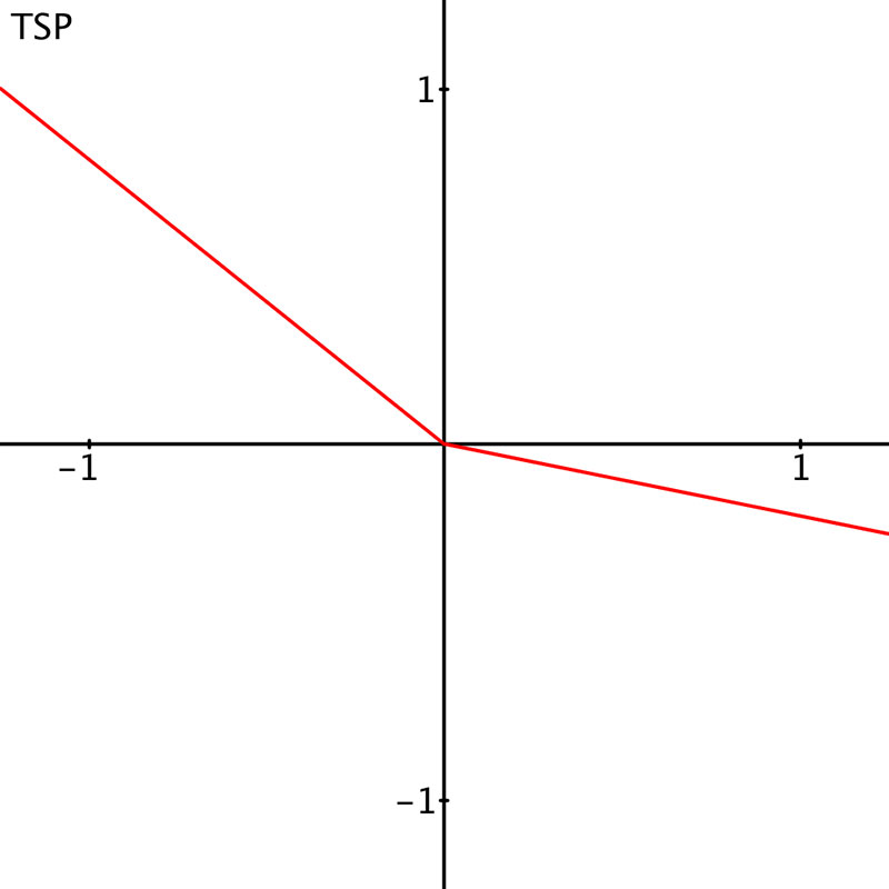
Figure 3. The Two Slope Parametric (TSP) activation function. TSP(x)=a*x when x<0, TSP(x)=b*x when x>=0. Each TSP function needs to be supplied with two parameters a and b.  In contrast, ReLU has no parameters to adjust. Different values of a and b provide a useful range of operations. If a and b are set to 1, then x = TSP(x); the TSP is a straight through connection. If a = 0 and b = 1, then TSP(x) = ReLU(x).

---

Combining the Concepts

Figure 4 shows a neural network layer where the fast transform is used as the system of weighted sums and the adjustable TSP activation functions allow the layer to be modified by a training algorithm to actually learn things.

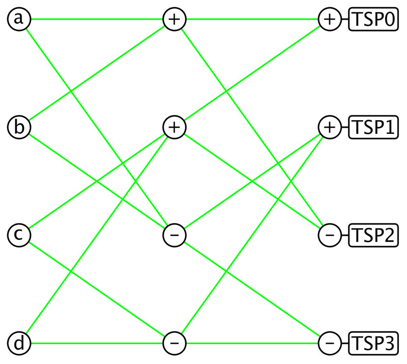
Figure 4. A lightweight neural network layer. Each green edge weight is one which leaves just four add and four subtract operations before the TSP activation functions. For a neural network of width n, nlog2(n)/2 add operations and nlog2(n)/2 subtract operations are needed before the activation functions.

---

Here’s a code example in JavaScript using the Processing P5 library:

1.    class FFBNet {
2.      constructor(vecLen, depth) {
3.        this.vecLen = vecLen;
4.        this.depth = depth;
5.        this.scale = 1.0 / sqrt(vecLen);
6.        this.params = new Float32Array(2 * vecLen * depth);
7.        this.flips = new Float32Array(vecLen);
8.        for (let i = 0; i < vecLen; i++) {
9.          this.flips[i] = sin(i * 1.895) < 0 ? -this.scale : this.scale;
10.        }
11.        for (let i = 0; i < this.params.length; i++) {
12.          this.params[i] = this.scale;
13.        }
14.      }
15.    
16.      recall(result, input) {
17.        for (let i = 0; i < this.vecLen; i++) {
18.          result[i] = input[i] * this.flips[i];
19.        }
20.        let paramIdx = 0; // parameter index
21.        for (let i = 0; i < this.depth; i++) {
22.          wht(result);
23.          for (let j = 0; j < this.vecLen; j++) {
24.            const signBit = result[j] < 0 ? 0 : 1;
25.            result[j] *= this.params[paramIdx + signBit];
26.            paramIdx += 2;
27.          }
28.        }
29.        wht(result);
30.      }
31.    }

Line 1 is the class declaration. Line 2 is the constructor declaration; vecLen is the width of the neural network and has to be some power of 2 (2, 4, 8, 16, 32 …) to match the requirements of the WHT. The depth term indicates the number of neural network layers.

Lines 3 and 4 store the information in the constructed object. Line 5 provides a scaling factor for the WHT that causes it to leave the vector magnitude unchanged.

Line 6 declares an array of parameters for the TSP activation functions used in the network. This is the adjustable part of the network. Line 7 sets up an array of sign flips used to prevent the first WHT from taking a spectrum of the input data, which with natural data like sound or images would cause some unwanted initial bias.

Lines 8 to 10 set up a sub-random pattern of sign flips and also incorporate a scaling factor for the last WHT used in the network. The conditional operator ? is used to select between two choices.

Lines 11 to 13 initialize the network with both slopes of each TSP function set at 45 degrees after allowing for the fact that a scaling factor for each WHT is incorporated. Initially, the TSPs allow information to flow through unchanged (aside for the scaling factor) which could be termed zero curvature initialization. This seems to help training of the neural network substantially.

Line 16 is the neural network recall function or feedforward function where you supply input and result arrays of size vecLen as decided in the constructor.

Lines 17 to 19 copy the input array to the result array with spectrum breaking sign flips and a WHT scaling factor. All further processing happens in the result array.

Line 20 sets the TSP activation function parameter index to zero. The index is increased by two for each individual TSP activation function since each TSP selects between two possible slopes.

Line 21 is the neural network layer count for loop.

Line 22 calls the WHT function which is used as a fixed collection of weighted sums. The cost of the transform is nlog2(n) add subtract operations, plus indexing and memory access costs. That is still much lower than the n squared multiply add cost of the weighted sums in a conventional neural network layer.

Line 23 iterates over all the individual parameterized TSP activation functions needed for this layer.

Line 24 decides which of the two slopes to apply based on whether the input to the TSP function is less than zero or greater than or equal to zero.

Line 25, the input to the TSP, is multiplied by the chosen slope.

Line 26, the parameter index, is increased by two, ready for the next TSP activation function.

Line 29, a final WHT, is applied to the result as a pseudo-readout layer, improving the behavior of the network at little cost.

Training Options

There are several options to train lightweight neural networks. Since a low number of parameters are involved, mutation-based training is possible as an alternative to the more usual back-propagation type training.

Online training where the neural network learns from immediate incoming data is also possible. In the source code included in the downloads for this article, three training options are provided.

Training with Sparse Mutations

This is ideal where you have a fixed training set for the neural net. If the training set is large enough and has some consistency between the inputs provided and the neural network outputs required, then the network has a good chance of generalizing well.

Training with Gaussian Noise

This can work well for online training where you can evaluate and choose between mutated and non-mutated network responses to some immediate piece of information.

It also works well for fixed training data sets. The main difficulty is setting the ideal mutation rate which may require some experimentation.

Training with Backpropagation

This is the fastest method and can be used for both fixed data set and online training. The main disadvantages are uncertain numerical stability and weaker generalization than you get with the mutation-based training methods.

The example code has mostly been written using Processing. Processing is a coding and editing environment for rapid code prototyping in JavaScript, Java, and some other programming languages.

Example code showing all three modes of training in Processing JavaScript and Java have been provided in the downloads.

The sparse mutation training method is demonstrated using straight JavaScript and Java as well.

A Maze Example

To demonstrate that lightweight neural networks can learn and show useful behavior, a maze escape problem has been coded. An agent (a yellow circle; see Figure 5) is placed in the middle of a maze.

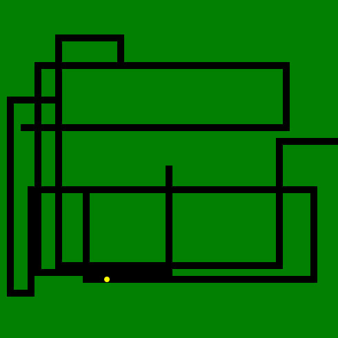
Figure 5. An agent controlled by a lightweight neural network tries to escape a maze.

---

It can see one step ahead, behind, above, and below, which is not an abundant amount of information. It must decide which way to go, remember which way it’s going, where it has been, etc.

It also has to learn to do all those things from scratch. The neural network is set up to work recurrently which provides a certain amount of working memory to the system.

Training is carried out on 200 randomly generated mazes using the sparse mutation method.

The agent is given two reward signals: how far it has managed to get from the center of the maze; and if it has managed to escape from the maze.

It’s allowed 300 time steps to escape. Some choices have been made about the size and depth of the neural network, which you can alter along with any of the other parameters.

If you run the code and let it train for a while, you can see the agent does develop at least some maze escape capability.

Good luck with your training and lightweight neural networks!  SV

---

Resources

---