---

Part 3: Transitioning to Real Hardware

The first installment of this series examined reasons why LiDAR could soon replace the ultrasonic and infrared ranging sensors that have typically been used for navigation on many hobby robots. The second installment used a simulation to show that an analysis of LiDAR data could isolate objects in the room and categorize them based on their size and position relative to the robot. This allowed a simulated robot to navigate through a known environment by identifying various obstacles and moving toward them. This article explores how to transition the simulation-tested ideas discussed in the last article to real LiDAR hardware.

The LiDAR simulation from the last article assumed the LiDAR data was a series of vectors as shown in Figure 1.

FIGURE 1.

---

The magnitude of each vector is the distance to objects or walls within the robot’s view or the maximum allowed distance if no objects are within range at that particular angle. The different colors in Figure 1 indicate the various objects identified by the robot (see the last installment in this series for more information).

Storing this data as vectors (an angle and distance) seemingly would be an obvious choice because of the way LiDAR data is obtained (distance readings are taken at various angles). Most LiDAR systems, though, store this information as the x,y coordinates of the vector endpoints as shown in Figure 2.

FIGURE 2.

---

Obviously, it’s equally valid to store this information as either a vector (the angle and length of the measurement) or by the coordinates of the endpoint (x,y). When stored as coordinates, the collection is generally referred to as a point cloud.

Since each data point is actually obtained in vector form, you might wonder why they are typically converted to coordinates. The reason is that LiDAR data is generally used to create a map of a robot’s environment, and the mathematics for doing so is easier if coordinates are used. Some systems — like the LiDAR in the Neato robotic vacuum cleaner — actually store the data as vectors because they use the information to analyze obstacles instead of mapping the room. Since the system discussed in this series of articles is also just detecting and analyzing objects, our preferred format will be vectors.

Hybo iLiDAR

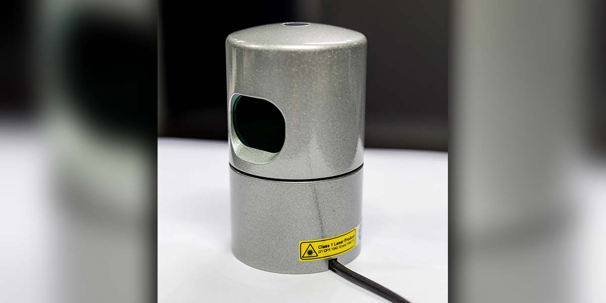
Before purchasing LiDAR hardware, I researched a number of different units and settled on the Hybo iLiDAR shown in Figure 3. I found it on Kickstarter and chose to back it because of its solid-state design. Unlike most LiDAR systems, it has no moving parts and I really liked the idea that there was no continually rotating motor to worry about.

FIGURE 3.

---

The manufacturer has had several delays, mostly because of calibration issues and some problems meeting some of the initial specs. They have always kept backers updated though, and even offered refunds to those that wanted them.

When they started getting close to the finalized unit, they were looking for beta testers and I volunteered. I enjoyed the process because it gave me access to a lot of early information, as well as being able to offer input on problems I found. All in all, I’m very pleased with the unit I tested, and expect to get my final production version before this article is published.

Demo Program

My goal for this article was to generate a demo program that would implement the object analysis discussed in Part 2 of this series using live LiDAR data instead of just a simulation. Some problems were encountered, so I’ll also discuss why these occur and how I solved them.

The main program for the demo is shown in Figure 4. It’s written in RobotBASIC: a language I helped develop and give away free at www.RobotBASIC.org. Each functional section of the code is grouped in a standard BASIC subroutine or in a callable sub-routine.

FIGURE 4.

---

This should make it easier to understand various aspects of the code in case you want to make modifications or translate it to another language.

The variable LidarHardware can be set to TRUE if you have the Hybo hardware. Setting it to FALSE forces the program to use a sample data file instead of obtaining a live scan from the hardware. This makes it easy for those without the hardware to experiment with the program.

Next, we’ll look at some of the modules used in the main program.

The Setup module shown in Figure 5 creates three arrays that hold the three-dimensional point cloud obtained from the LiDAR (only the x and y values will be used), the vectors that will be used for our analysis, and the object data created by the analysis. There are also some global variables that control how far the LiDAR will scan and the width of the scanning range as well as others discussed in the previous article.

FIGURE 5.

---

The LidarScan module (see Figure 6) needs to obtain the point cloud data directly from the LiDAR hardware. Often this can be a very complicated problem because most LiDAR units are continually scanning and therefore continually sending data. Generally, your software has to watch for special sequences of bytes to determine where the data begins, and this often has to be repeated numerous times in case the special sequences just happen to occur in the point cloud data.

FIGURE 6.

---

When I was working as a beta tester, I suggested that they create a stand-alone program that could perform all that grunt work for you, and obtain a single data scan and store it in a disk file using Microsoft’s Excel comma delimited format (.CSV). This makes it very easy to obtain the LiDAR data as shown in Figure 6.

Once the program SensorToCSV has been spawned, it obtains the point cloud data and stores it into a disk file named MyData.csv. Other modules (also shown in Figure 6) read the disk file and convert it to a vector format using some simple trigonometry.

The vector format needed for my analysis assumes that the vectors are stored in the array V[] in ascending angular order. Since the simulation discussed in Part 2 of this series demonstrated that there is no need for a resolution better than one degree per reading, the code shown automatically removes duplicate integer angles as well as data points that might be invalid.

The modules shown perform all the major functions of this program. Other modules called from the main program simply graph data points, and calculate and display object data as discussed in Part 2 of this series. This new FindObject module has been improved so you can look for an object that is smaller than some maximum, as well as larger than some minimum value.

When working in a real world environment, this modification proved to be helpful. Adding the ability to search on distance criteria (find the closest object, for example) might also be valuable, but I have intentionally kept things simple for this article.

Limitations

As we’ll see in an example scan, there are some limitations that need to be mentioned. First, most LiDAR units do a full 360° scan (which itself can be a problem unless the unit is mounted on top of the robot). The Hybo iLiDAR only scans 180° because of the solid-state constraints. Furthermore, a few points at each end of the 180° window might be inaccurate or invalid.

This limited scan angle can increase the time needed to map a room, but it does not present a problem for our purposes. In fact, when searching for objects, it can often be beneficial to limit the scan angle to 140° or so (from -70° to +70° from the robot’s current heading). If you recall from Figure 5, you can set the variable ScanWidth to control the range of angles as you see fit.

The simulated scans in Part 2 always have perfectly reflective simulated objects to analyze. In the real world, there are objects such as mirrors, plants, furry pillows, etc., that can create unpredictable reflections and thus unusable data.

Usually, this can be solved by doing something simple such as adjusting the path you want your robot to follow or limiting the scanning angle or maximum distance.

During experimentation with the iLiDAR hardware, I occasionally found a data point whose angle was inconsistent with points around it. Most of the time, such points would play havoc with my program’s analysis. Once I found the problem, though, it was easy to detect such situations and simply ignore them when converting the point cloud data to vectors.

Real World Examples

Now that you have a better understanding of how the program works, let’s see it in action to demonstrate some of the points that have been made. Figure 7 shows an experimental environment situation created in my home. Notice that there are three white objects in view as well as a wall of cabinets. These should all produce great reflections.

FIGURE 7.

---

Figure 7 also shows a wicker basket near the left side of the cabinets. To the left of the basket is an end table with another basket sitting in an open area below the table surface. Notice the coffee table in the lower left hand corner of the picture. It has three legs on each side with significant amounts of open areas. Each of these objects have the potential for detection problems.

Figure 8 shows a graph of a point cloud taken about 12 inches above floor level. The simulated robot has been drawn on the screen to show where the real LiDAR unit was positioned. Labels have been added to help you identify the objects from Figure 7.

FIGURE 8.

---

Notice the basket — even with its irregular surface — was viewed fairly accurately. The open areas under the end and coffee tables, though, were at a height that did not reflect the LiDAR’s laser beam. The real question is how will the vector analysis that was used for the simulated environments deal with this real world data.

Figure 9 shows the results after translating the point cloud to vectors and analyzing the data to look for objects. It’s easy to relate each object found to the items in Figures 8 and 9. For example, object 4 is the basket and it’s 204 units away with a width of 12°. If we want to move toward the basket, the robot can face it by turning 24° to the left (see the object info in Figure 9).

FIGURE 9.

---

In this case, the maximum allowed range was 250 units (the blue arc). Notice how this restriction removes long-range objects like the white board and the items behind the end table from view. Sometimes this ability can be very beneficial. Constricting the scan width to 140° (±70°) prevented the coffee table from being seen since its open areas could potentially confuse the software.

Since the two white boxes were added to the environment for demonstration purposes, this example has more objects than you would normally expect to see. This makes the objects somewhat similar in size but a desired object could still be potentially recognized based on its position and distance from robot.

If you recall from the second article in this series, the purpose of finding objects in the robot’s view was to help with navigation. The idea behind this approach is similar to walking through your house at night, unable to see much more than general shapes.

Since you know what to expect when walking through your own house (a known environment), you can identify key objects using their position and general size and then move toward them to get to the next point in a pre-determined path.

Repeating this process until the desired destination is reached is an unusual but effective way to move between assigned positions in a known environment. Refer to the second article in this series for more detail on this process.

Conclusion

The conventional way of utilizing a LiDAR (SLAM, Simultaneous Mapping and Localization) is a powerful tool for many robotic applications. The ideas expressed in this series can be easier to implement for robots operating in known environments — especially if they have limited computing power and memory.

If you would like to delve into these ideas further, you can download the full program discussed in this article from the “In the News” tab at www.RobotBASIC.org.  SV

---