---

The previous articles in this series dealt with improving ultrasonic sensor performance — especially by using parabolic reflectors to focus the acoustical energy. Such a parabolic reflector mounted on the ultrasonic sensor and electronics is shown in Figure 1.

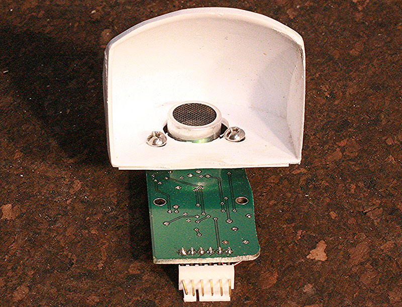
Figure 1. Ultrasonic sensor with parabolic reflector.

---

Focusing the energy with these reflectors narrows the sensor’s field-of-view, producing a collimated beam. That, in turn, means that a robot or other vehicle incorporating such sensors for collision avoidance (as an example) will not be responding to objects that never posed a threat in the first place.

We can improve the response of our ultrasonic-equipped vehicle still further by employing two ultrasonic detection sensors. These two sensors will have slightly different responses to the same object. We can exploit that difference to determine not only how far away the object is, but how far to the left or right it is. Before we do this, let’s look at why such a two-dimensional view is important.

Imagine that, instead of a microcontroller, you’re inside the vehicle with a single ultrasonic sensor as your only detection of the outside world. As you travel forward, the sensor alerts you to the fact that an object exists three feet ahead. What do you do?

You have several options: completely stopping; turning to the right; or turning to the left. Without any additional information, perhaps the best option is to slow down and make a hard left or right turn.

Given this limited intel, that’s the best we can do. So, what if the situation is as depicted in Figure 2? What if the vehicle is programmed to slow and make a hard right turn upon detecting an obstacle? In that case, it will be turning toward the obstruction (the wall) — not away from it.

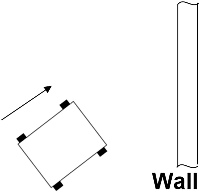
Figure 2. Vehicle approaching obstruction on its right.

---

What if the situation is as depicted in Figure 3? Here, the obstruction is a large object slightly blocking its left side. A simple quick turn to the right — even without reducing speed — is all that’s needed to avoid collision. Yet, with only the information that an obstruction exists somewhere in front of the vehicle, there is no way to be sure that such a simple procedure will avoid hitting the chair leg.

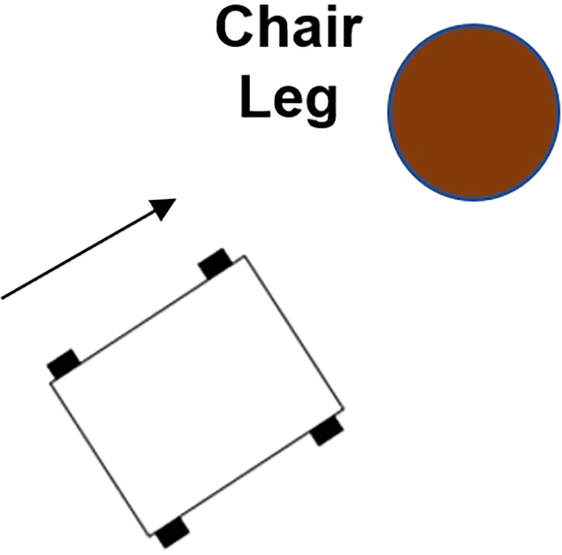
Figure 3. Chair leg obstruction.

---

Fortunately, radar designers solved this problem long ago. The answer is to incorporate two transmit/receive sensors located close to one another, as shown in Figure 4. The two transducers with centers d inches apart simultaneously transmit their ultrasonic energy in phase, and then individually receive the return energy. This is referred to as angle tracking.

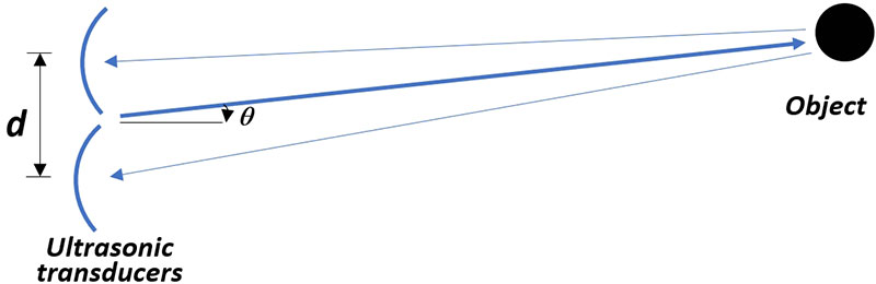
Figure 4. Angle tracking.

---

In the Figure 4 example, it’s obvious the returned energy travels a slightly greater distance to the bottom transducer than to the top transducer. Therefore, its time-of-flight (TOF) will be slightly greater. The ultrasonic energy is transmitted as a coherent wavefront and retains coherence during its travel. So, we will actually see the two signals at the sensors as sine waves with distinct phase and, in this example, with the phase of the bottom signal lagging the phase of the top waveform.

Note in Figure 5 that the blue (left) waveform arrives approximately eight microseconds ahead of the green (right) waveform, indicating the object is on the left. But can we determine just how far to the left?

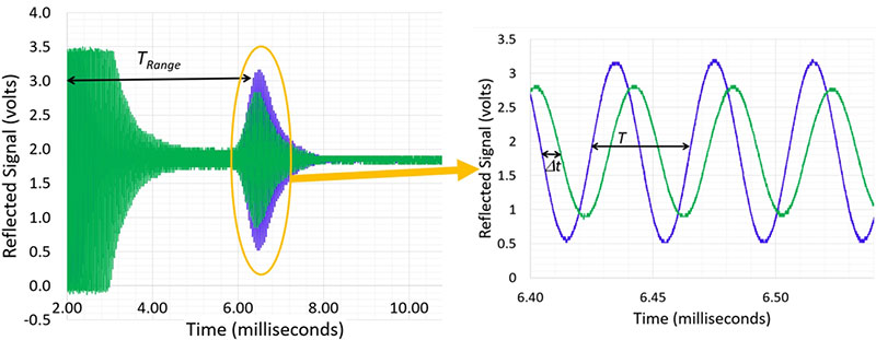
Figure 5. Reflected signals showing: a) full response; and b) zoomed in at the peak.

---

To analyze this, approximate the left and right rays as parallel lines as in Figure 6. As you can see, a right triangle can be constructed at the end of the two rays. The hypotenuse of the right triangle has length d, which is the distance between the two sensor centers. The longer ray (the bottom one in Figure 6) therefore exceeds the length of the shorter ray by d· sin(θ).

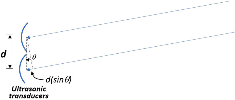
Figure 6. Analyzing the phase difference by approximating the two rays as parallel.

---

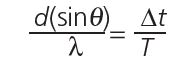
Dividing this product by the ultrasonic wavelength, λ, gives us the fraction of a cycle that the later ray lags the earlier ray. Look again at Figure 5 to see these two waveforms and the phase difference between them.

This fraction of a cycle can also be expressed as the time difference between those two waveforms divided by the period of the waveforms.

Equating these two ways of writing the phase difference gives us:

which can be simplified by recognizing that:

and

 c is the speed of sound in these equations (13,400 inches/second) and f is the frequency of the ultrasonic waveforms (25 kHz for the ultrasonic sensors in this build). Combining these equations results in:

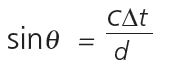
For the Figure 5 timing difference of ∆  t = 8 µsec and with a separation between the ultrasonic sensors of 2.5 inches, this becomes:

sin θ = 0.042

so

θ  =  2.5°

Now, the question is whether an object that is 2.5° from the front center of the vehicle (as shown in Figure 7) presents a potential collision.

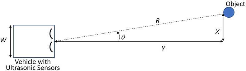
Figure 7. Determining the distance from center.

---

To determine this, we need to know how far the vehicle is from the object. This is just the range, R — a parameter that all ultrasonic ranging systems (by definition) measure.

It’s straightforward to calculate from the original ranging data. It’s just the time that it takes for the ultrasonic energy to reach and reflect from the object and make its way back to the sensor (T_Range in Figure 5a), times the speed of sound and divided by 2:

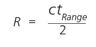
The factor of 2 accounts for the fact that the energy must make a round trip from the ultrasonic transceiver to the object and back to the transceiver before being sensed.

Once we know R, we can calculate the object’s distance, X, from the vehicle’s center:

X  =  R sin θ

If the vehicle’s width, W, is greater than twice this number, then the object is in its path and the vehicle must take the appropriate diversionary action.

In the Figure 5 example, T_Range is approximately 6.4 milliseconds, so R is about 43 inches. Therefore, the object is:

X  =  (43)(0.042)  =  1.8 inches

from the center axis of the vehicle. Thus, if the vehicle’s width is more than 3.6 inches, the object is in its path.

Note from Figure 7 that some objects (such as a round chair leg) may still be in the path of the vehicle, even though the tracking angle says they are marginally outside the boundaries of concern. This is because the main reflection will be from approximately the center of the object (in Figure 7, the part of the circle nearest the vehicle), even though part of the object is closer to the vehicle’s path. For this reason, it’s generally a good idea to expand the region considered within the vehicle’s path.

The Complete Ultrasonic Tracking System

So, that’s the theory. How do we implement this?

It’s simple, if you already know how to implement the single-sensor version of the ultrasonic ranging system described in the previous articles in this series. The angle-tracking version is simply two separate versions of the single-sensor system all the way to the microcontroller (a single microcontroller is common to both receiver sides).

Figure 8 is a block diagram of the dual-sensor version and Figure 9 is a photo of the completed board.

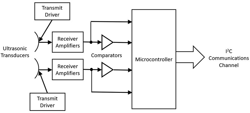
Figure 8. Block diagram of the dual-sensor angle-tracking ultrasonic system.

---

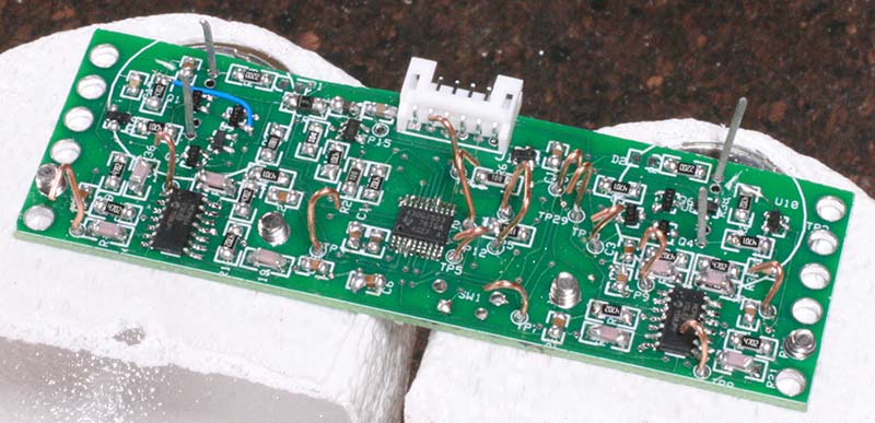
Figure 9. Circuit board (with testpoints) mounted to reflectors.

---

The microcontroller does the timing comparisons needed to compute range and offset at a rate of up to 50 times per second (on demand from the host). It takes these timing measurements and computes the range in inches (0 and 255) and the offset in inches (-7.9375 to +7.9375). It then reports these to the host via the I2C communications channel.

Although the individual functions shown in Figure 8 have been discussed earlier, it’s important that we make available a full schematic of the complete angle-tracking dual-sensor system. The schematic is too large to publish in this article but is available with the article downloads.

The other thing needed is a complete listing of the microcontroller program for the MSP430G2553 microcontroller used. Again, a printed version of the program would be too long for listing in the article but it’s also available with the downloads.

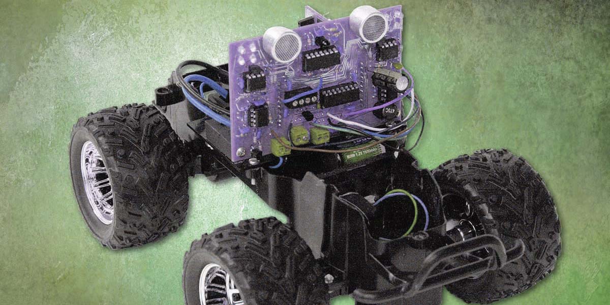
Figure 10 depicts the final version of the angle-tracking sensor mounted on an experimental vehicle (the electronics are below the reflectors, hidden by the black pedestal on which the assembly is mounted).

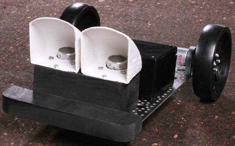
Figure 10. The final dual-sensor angle-tracking ultrasonic system mounted on a small vehicle.

---

Series Conclusion

I hope this series of articles has provided a better understanding of ultrasonic device theory — especially the challenges of using that kind of acoustic energy for detection, and the solutions that are available to make ultrasonic detection a reliable repeatable source of detection.

These solutions especially include the use of parabolic reflectors to focus the energy: making the energy a collimated, more intense beam within a controlled boundary; and the use of dual sensors as a means of estimating the direction (in addition to the range) of reflections sensed by the system.  SV

---