---

Receiver and Control Electronics

So far, we’ve covered the basics of piezoelectric transducers, the transmitter electronics for driving the transducers, and the improved focusing of that ultrasonic energy into and out of the transducer using parabolic antennas.

The original intent was for this to be the final article in the Ultrasonic Radar series. In addition to covering the receiver and microcontroller for the project, it was to go into detail about how to create a two-dimensional radar that computes not only range but also the bearing (that is, direction). However, the two-dimensional radar topic really needs to be an article by itself, so that will be covered next time.

The Receiver

One of the challenges in designing an ultrasonic receiver is the fact that the dynamic range of the signal is large. When sensor designers refer to dynamic range, they’re talking about the ratio of the largest received signal to the smallest received signal.

As mentioned in previous articles, the use of a parabolic antenna minimizes this dynamic range by focusing the ultrasonic energy into a narrow cone that is virtually a cylinder. As a result, the energy loss as a function of distance from the transducer is fairly small. However, once the energy strikes the object, it will be reflected in different ways.

A flat, hard, “smooth” surface will reflect the energy back in a “specular” fashion (Figure 1a). Other surfaces will reflect the energy back in a “diffuse” manner (Figure 1b), spreading the energy out.

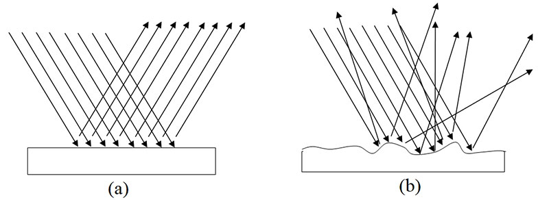
Figure 1. (a) Specular and (b) diffuse reflections.

---

A specular reflection “bounces” all the energy in a mirror-like way, while the diffuse reflection scatters the energy.

“Smooth,” in this case, is a function of the surface variation relative to the wavelength of the energy (for 40 kHz ultrasonic energy, the wavelength is approximately 0.33 inches). A surface with variations much greater than one wavelength would definitely be rough, and a surface with variations much less than one wavelength would definitely be smooth.

So, the reflected energy echoed back to the receiver is not only a function of distance (as we already know), but a function of the object’s surface and geometry. In addition, the orientation of the object to the sensor also plays a role.

The bottom line for all this discussion about smoothness, object geometry, orientation to the receiver, etc., is that the received signal will vary considerably. The received signal can easily vary by a factor of 500 over the range of, say, one foot to 20 feet.

Handling a Large Dynamic Range with a Microcontroller

Okay, so we need to design for a large range of signal values. How might we handle that? Let’s recognize that we’re going to incorporate a microcontroller in our design, and most modern microcontrollers have multiple analog inputs.

One way to digitize a large range of values with a fairly simple design approach is to cascade two or three amplifiers as in Figure 2.

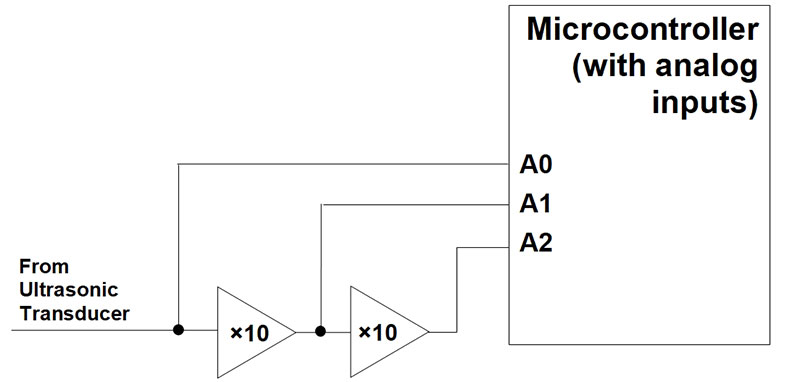
Figure 2. Cascaded amplifiers provide extended dynamic range.

---

Each of the amplifier outputs can be sampled and digitized. We can use the output of the first amplifier for signals that are at short distances, and use the second or third amplifiers at the longer distances.

Amplifiers are easy to design using op-amps. For an inverting amplifier, the gain is given by -R_ƒ/R_i and for a non-inverting amplifier, the gain is 1+R_ƒ /R_i. If each of three stages has a gain of 10, we can digitize just about any valid signal coming from an object as far away as 20 feet while achieving sufficient accuracy with the analog-to-digital converter (A/D; typical microcontroller A/Ds have about 10 bits of resolution).

In many cases, we’ll want to AC-couple the individual gain stages. This keeps small DC offsets at the input to the cascaded chain of amplifiers from being multiplied by the gain of each stage. For an inverting amplifier, AC-coupling is as simple as just adding a capacitor before the input resistor of the amplifier.

How Does Feedback Work with an Op-amp?

A feedback amplifier using an op-amp is a powerful design component for most analog applications and its operation is straightforward. Let’s start with an op-amp and write down a few characteristic equations for it (Figure 3).

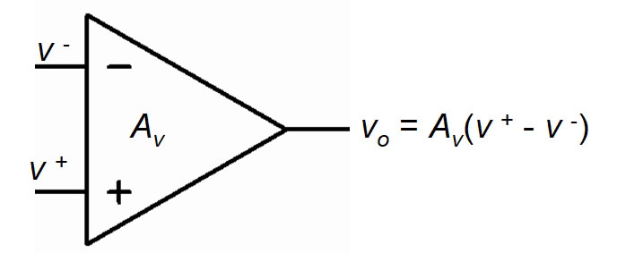
Figure 3. Op-amp with gain of A_v.

---

An ideal op-amp has high impedance inputs that allow no current to flow into them, so the important equations are just:

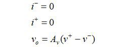
So, the output voltage is equal to the difference between the input voltages multiplied by the op-amp’s (usually quite large) voltage gain, A_v. That’s all we need to know (at least for this ideal case) about the op-amp.

Let’s analyze an inverting amplifier (Figure 4) just to see how this works.

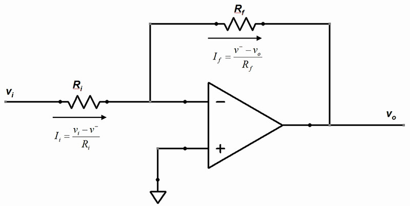
Figure 4. Inverting amplifier.

---

We’ll add a couple of resistors. One of these, R_ƒ, feeds back the output voltage to the negative input terminal. The input resistor, R_i, is connected between that input terminal and the signal. Since the op-amp inputs do not allow current in, the current through the feedback resistor, I_ƒ, is equal to the current through the input resistor, I_i:

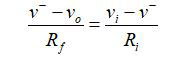
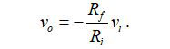
Since v⁺ = 0, then v^- = -v_o /A_v, resulting in:

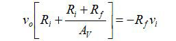
Also, since A_v is typically a very large number (10³ < A_v <10⁶⁾:

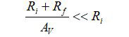
For most practical feedback amplifiers, this equation can be simplified to:

Getting By with Just One Power Supply

The Figure 4 schematic shows a ground reference at the non-inverting input. This circuit (as with many shown in examples) assumes that the power supplies to the op-amp are two equal, but opposite-sign voltages; for example, +12V and -12V. Such relatively high bipolar voltages were the norm in earlier times.

In modern microcontroller applications, the microcontroller and other digital functions are typically powered from +3.3V or a similar single low voltage. A dual supply — particularly like the traditional ±12V setup — is inconvenient; both because of the higher voltages required and because a negative voltage is needed. Fortunately, many modern op-amps are capable of operating from voltages in the 3V to 5V range.

To do this, we use the +3.3V (or whatever voltage level we are using) as the positive op-amp supply voltage and use ground as the negative supply voltage. We create a voltage that’s about half of the positive supply voltage and reference all voltages to that. How does that work?

Let’s take another look at the inverting amplifier, but this time using a single supply voltage (Figure 5).

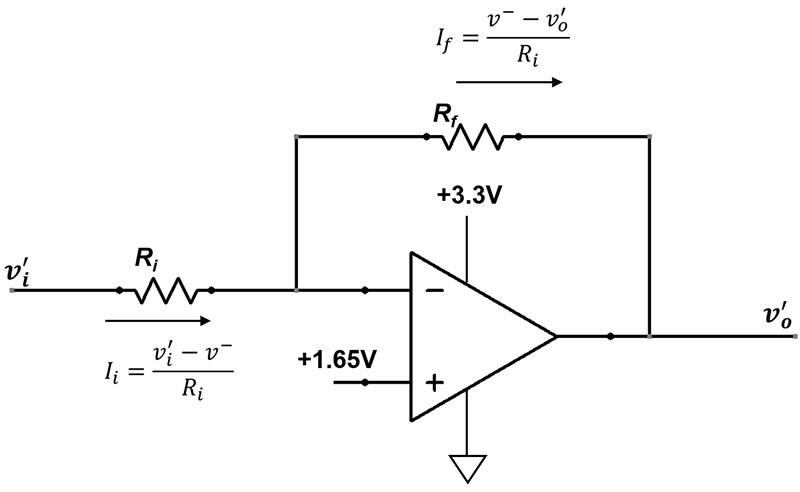
Figure 5. Single supply inverting amplifier.

---

The input voltage, v_i^’ has the apostrophe added to indicate that it has a 1.65V DC pedestal. That is:

We’ll also use v_o^’ to indicate that it could have a DC level added, although we haven’t determined yet what that DC level is. Again, using the fact that I_i = I_ƒ the resulting voltage equation is:

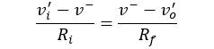
We eliminate v^– by using the op-amp relation:

to get:

The Figure 5 circuit applies gain only to the original (no DC pedestal) signal and preserves the 1.65V pedestal at the output. In this way, an entire board full of analog circuits can operate from a single power supply while using a reference that is halfway between the supply voltage and ground.

In many instances, the mid-level reference can be achieved with just a two-resistor voltage divider. Although, in instances where the reference must sink or source current, it may need to be buffered by a voltage follower.

Setting the Threshold for Detection

An important consideration in designing receivers of this sort is what to make the threshold. What signal amplitude is high enough to indicate that an object is reflecting back?

With conventional aircraft radar, the method usually adopted is to choose a threshold that is some multiple of the noise amplitude. Signals at this threshold voltage will have a signal-to-noise ratio that produces a sufficiently low probability of a “false alarm” (that is, a false detection of an object). This approach to setting the threshold is known as Constant False Alarm Rate (CFAR).

In the case of our ultrasonic sensing, the random noise that is referred to when people talk about signal-to-noise is so very low that we typically don’t need to worry about it. Our main concern will instead be offset voltage which — for typical op-amps (that is, an input offset of 1 mV) and with a gain of 10 — will be on the order of 10 mV maximum at the output, regardless of which amplifier stage is used (because the stages are AC-coupled to one another).

A threshold on the order of 100 mV should provide good probability of detection while making probability of a false alarm quite low.

The I²C Interface to the Ultrasonic Sensor

The MSP430G2553’s I²C interface is fairly straightforward and is well-documented in TI literature. In addition, there have been some very good explanations of the I²C protocol in this magazine, so the description here is just a high-level summary.

The I²C interface has just two signals. One of these, SDA, contains the data while the other, SCL, serves as the clock. These two signals also initiate and terminate data transmission and perform other special functions in addition to their data and clock roles.

Note that, unlike SPI (Serial Peripheral Interface) or RS-232 and its variants (usually just referred to as “serial links”), the data line in I²C is bidirectional. In order that all the devices connected to the data line can use that single SDA line for both input and output, the line is “pulled up” with a resistor to the supply voltage and the individual I²C transceivers can then pull the line low with their output transistor (a logic ‘0’), or leave the line pulled up by leaving the output transistor off (a logic ‘1’).

To orchestrate the activity between devices, one I²C device is designated “master” while all the other devices are “slaves.” The master generates the clock and makes sure that only one slave talks at a time.

Another very helpful feature of I²C is the fact that the addressing of nodes is built into the protocol. Each slave node has its own unique address; that way, the master can designate which slave it wants to talk to.

What’s Next?

The final article in this series will discuss the details of getting the ultrasonic radar to detect not only range but bearing as well. In addition, the full schematic and the assembly language code for the radar will be included.  SV

---

---

---