Stabilizing an Inverted Pendulum

Stabilizing an inverted pendulum is a favorite and much discussed control theory problem for roboticists.

The basic idea is illustrated in Figures 1 and 2.

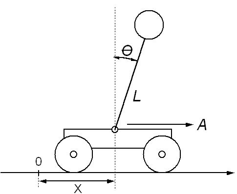
Figure 1. An inverted pendulum connected by a free pivot to a motor driven robot base.

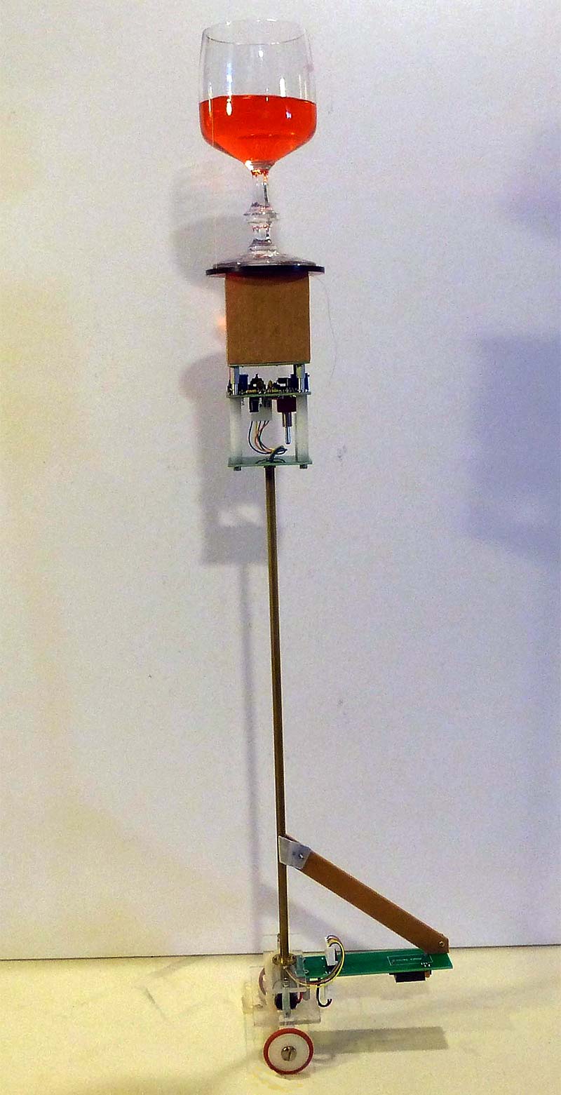
Figure 2. Balancing a glass of wine without getting tipsy!

Simply put, the problem is to drive the robot base forward or backward in such a manner as to prevent the inverted pendulum design from falling over. In this article, we’ll explore the math and science behind this seemingly simple task.

As an Electrical Engineer at Union College in 1965, this was my senior year project. I had nine months to apply classical control system theory (Laplace transforms, Bode plots, Nyquist criterion, Root Locus, etc.) to analyze the problem and then build a working model.

For computation, I had my slide rule and the privilege to use the first computer ever to arrive at Union College: the IBM 1620. A marvel of the age, it clocked at 100 kHz, and boasted a 20K nib memory (a nib is four bits) — all for only $65,000.

My primary resource for electrical and mechanical components was a basement full of WWII surplus goodies; many from the B-29 gunnery control system. My 28V “cart” drive motor originally fed bullets to one of the two machine guns in one of the four turrets spread around the B-29. I powered this motor with an amplidyne: an electromechanical motor generator pair that could amplify 20 mA from a vacuum tube into 2 kW to drive the motor that rotated a gun turret.

Decades ago, the first really important application of the inverted pendulum problem was stabilizing a rocket on its thrust vector. Today, with the availability of inexpensive gyroscope and accelerometer chips, stabilized inverted pendulums are very common; most notably, the Segway, balance boards, and self-balancing toys like the MIP and Mipasaur from Wowee.

Numerous analyses of the problem can be found online; some running to 70 pages of fairly dense mathematics. Is there a way to solve this stabilization problem with just plain common sense and a little intuition? That is what this article hopes to do with nothing more than high school level physics.

First, let’s get a little flavor of the classical method that I applied in 1965. A system like the motor driven inverted pendulum can be represented by complex numbers plotted on a Root Locus diagram like that shown in Figure 3.

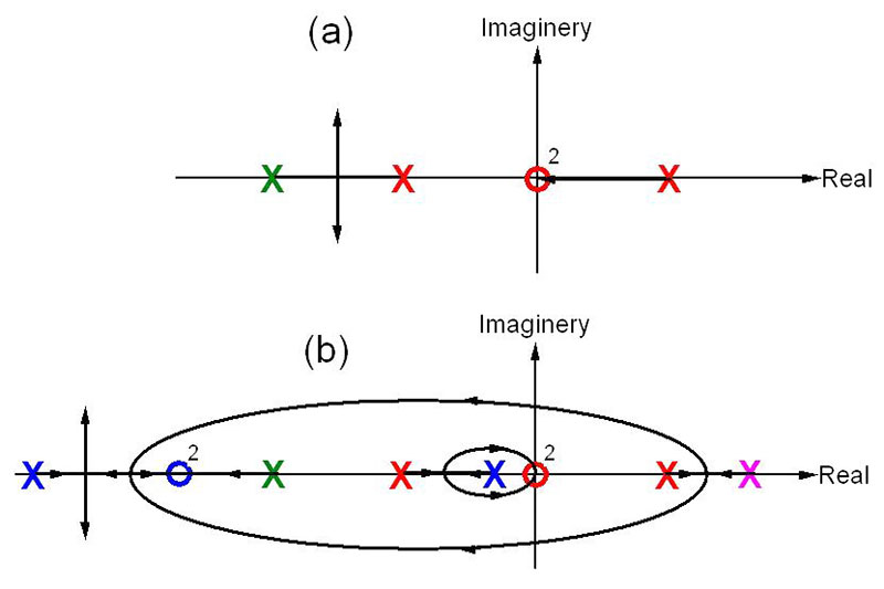
Figure 3. Root Locus diagrams for the motor driven inverted pendulum stability problem. The red poles/zeros represent the inverted pendulum; the green pole is the motor drive response; the purple pole is the instability from the unstable position control loop; and the blue poles/zeros are the stabilizing compensation function. The small 2s indicate two zeros at the same point.

In this diagram, the frequency dependent characteristics of each component are represented by “poles” (shown by Xs) and “zeros” (represented by circles). For example, a charging capacitor with an RC time of 0.1s would show as an X at -10 on the real axis. Poles with an imaginery component (off the real axis) always come in matched upper and lower pairs, and represent oscillating behavior such as a pendulum or LC circuit. A stable oscillator with frequency w = 5 Hz would be represented by poles at ±5 on the imaginery axis. Any pole in the right half plane indicates instability.

In Figure 3a, the poles/zeros of the inverted pendulum are shown in red; for the motor drive, they are shown in green. When the feedback loop is closed — that is, the pendulum angle is amplified and applied to drive the robot base (referred to as “cart” going forward) motor — the poles move as a function of the loop gain according to complex (but well-known) rules as shown by the arrows. The path of the poles is known as the Root Locus.

One of those rules states that a pole tends to move toward a zero as gain increases, but can never pass it. The right half plane pole in Figure 3a (representing the inverted pendulum instability) can never escape the right half plane because of the two zeros at the origin. It cannot go up and over the origin because poles with an imaginary component must come in pairs, and we have only one pole in the right half plane. So, there is no value of gain for which this closed-loop system can be stable.

Figure 3a suggests two steps in the path to stability: (1) We need a second pole in the right half plane so that the two poles can come together, break away from the real axis, and make their way into the left half plane; and (2) We need to add some zeros in the left half plane to attract the two unstable poles.

Figure 3b shows in blue and purple how to add three more poles and two more zeros to achive the desired stability. The left half plane blue poles and zeros can be implemented with a single operational amplifier (op-amp) and a few resistors and capacitors. So, what about that additional purple pole in the right half plane. That means more instability. What is that all about?

If that control theory discussion leaves you confused, you are not alone. In 1973, I was asked to give a talk on the inverted pendulum problem for a group of engineers and physicists. In 40 minutes, I went through the discussion above with a lot more details and equations.

At the end of the talk, it was clear that I had not conveyed any intuition about the problem, and few understood the basics of the solution.

Now, skip ahead 45+ years when I happened to Google “inverted pendulum” and found lots of differential equations and complex diagrams but — again — no simple intuitive way to understand the solution. The Wikipedia article I came across derived equations for the dynamics of the cart pendulum system, but offered no clues on how to stabilize it.

What follows is my attempt to fill that void. My inspiration for a simplified explanation came from an article on the problems that crane operators encounter with swinging loads. I suddenly realized that the crane problem might be related to the inverted pendulum problem, and indeed it is.

Let’s begin by looking back at Figure 1 in which the three important variables of the system are the cart position X, cart acceleration A, and pendulum angle q.

Most of the basics of the balancing problem can be understood by considering human responses in the task of balancing a pole on the palm of your hand. If the pole is falling to the right, you need to move your hand to the right faster than the pole is falling (and vice versa) in order to “catch” it.

If the angle of the pole is q (radians), the mass at the top of the pole will be accelerating away from vertical at A = g q (g = acceleration of gravity = 9.8 m/s²), so your hand will need to accelerate faster than g q; perhaps 5 g q. Following this idea, a proposed control system to keep the pendulum from falling over is shown in Figure 4.

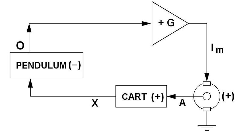
Figure 4. A proposed control system to balance an inverted pendulum. Note the sign of each component. Positive current Im to the motor produces a positive cart acceleration A. Positive acceleration will tend to make q decrease, so the pendulum block has a negative sign. Counting signs around the loop, we have one negative sign so the loop gain is negative — the normal situation for a feedback control system.

The angle q is sensed, amplified with gain G, and applied as a current I_m = G q to drive the cart motor. The motor produces the cart acceleration in the direction to reduce q. This is a feedback control system with the goal of maintaining q » 0. Unfortunately, as we demonstrated in Figure 3a, there is no value of G for which this system can stabilize the pendulum. It may zip back and forth once or twice, but the pendulum always falls over in a second or two as the cart races off the end of its track.

Since most people can easily learn to balance a pole, the human brain must be subconsciously doing something more complex than a linear response to the tilt of the pole.

Now, we come to the problem of the crane operator transferring cargo from dock side to the hold of a ship. He lifts the load from the dock and swings the crane over the hold. The result is a dangerously swinging load that cannot be safely lowered. Experienced crane operators learn to avoid this problem by moving the crane so as to prevent the oscillation.

Seen from the engineering point-of-view, this is a system with a strong resonance at the pendulum radian frequency:

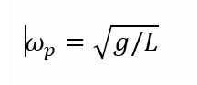
where L is the length of the cable supporting the load. If the frequency spectrum of the crane motion contains a component at w_p, the load will end up swinging.

The solution is to place a band suppression filter with center frequency w_p between the operator’s joystick and the position control of the crane. Modern cranes include this stabilizing feature.

In one of the beautiful symmetries of nature, this same band suppression filter — inserted in the signal path between the angle sensor and cart motor — solves most of the stability problem of the inverted pendulum. With this improvement, the pendulum may stay up for many seconds, but always ends up drifting ever faster away from track center.

Eventually, it will reach its maximum speed or the end of the track, and down goes the pendulum.

This remaining difficulty can be analyzed by considering the measurement of the angle of the pole from the vertical as defined by gravity. We do this with an angle sensor between the track and the pole, assuming a level track. However, the track will never be exactly level. If the cart tries to maintain an angle that is not perfectly vertical, it must — on average — accelerate away from its starting position.

For example, if the track is one millimeter out of level in a three meter length, the cart will run off the end of the track in 30 seconds or less. An offset of one minute of arc in the angle sensor zero has the same effect.

This problem is solved by adding a second sensor to measure the position of the cart and then modulating the null angle j (the angle the cart tries to achieve; nominally zero) by the difference between where the cart is and the center of the track. If the cart is left of center, shift the null angle slightly to the right. If it is right of center, shift the null angle to the left; that is, set the null angle to j = -kX where X is the cart position and k is a small adjustable constant.

This causes the cart to seek a position in which the null angle is perfectly vertical or right of center by whatever amount is necessary to exactly cancel any offset in the angle sensor and/or track slope.

There is an added bonus. Now, the position of the cart can be controlled by deliberately adding an offset to the null angle; that is j = -k (P + X) where P is a command position.

Now, the control system has two goals: keeping the pole vertical and maintaining a command position. Clearly, the vertical pole requirement must have priority, so the angle control loop must be faster and have higher gain than the position control loop.

Now it gets interesting. Imagine that — with the pole stable and vertical at track center (X=P=0) — we command a move to the right (for example) by suddenly increasing P from 0 to +0.1 meters. So, j suddenly becomes slightly negative which will cause the cart to accelerate to the left — the wrong direction!

The null angle modulation strategy results in positive feedback in the position control and will make the cart respond to a position command in the wrong direction!

This counter-intuitive situation can be understood by again considering human actions in the pole balancing task. If you want to move right, a starting move to the right will cause the pole to fall to the left. To avoid this, make a quick move left to produce a little angle to the right, and then chase it back to vertical by moving right.

This answers the question posed above about the requirement for a second source of instability. The position loop is set up with positive feedback which is represented by the purple pole in Figure 3b.

The final control system is shown in Figure 5.

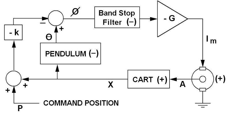
Figure 5. A control system that includes position control and a filter (the blue pole/zeros of Figure 3b) to suppress cart motion at the pendulum frequency.

In this diagram, the filter and final amplifier have negative gain because they will be implemented with inverting op-amps.

Note that the angle (inner) loop has three negative signs, so the loop gain is negative as expected for a feedback control system. The position (outer) loop has four negative signs causing positive feedback that would normally make that loop unstable if not for the stabilizing effect of the inner loop.

Now, at last I had a clear, simple, and intuitive explanation for the requirements to stabilize the inverted pendulum. I shared my thoughts by editing an abbreviated version of the ideas above into that Wikipedia article.

Building the Test Model

First, about that 1965 senior EE project: It did work (very well, actually), but it needed an umbilical cord connecting the cart to 60 pounds of vacuum tube electronics on the bench. With today’s electronics, it is easy to make it all self-contained.

Figure 1 illustrates the inverted pendulum on a two-axle four-wheel cart. However, it is more visually interesting to use a single axle two-wheel cart as shown in Figure 2.

In this case, the single axle is the pivot of the pendulum. The angle q between the pendulum and track is measured by mounting a distance sensor on a lever arm, facing down at the track a few cm in front of the pivot point. As q changes, the distance between the sensor and the track changes proportionally.

There are multiple ways to measure the cart position; for example, counting wheel rotations or using a slider on a resistance wire along the track. Since the voltage across a DC motor is nearly proportional to its rate of rotation, the cart position can also be measured by simply integrating the motor voltage. This is a simple method to measure the cart position as we design the circuit for our test model.

The schematic diagram of an analog control system implementing these ideas using three op-amps is shown in Figure 6.

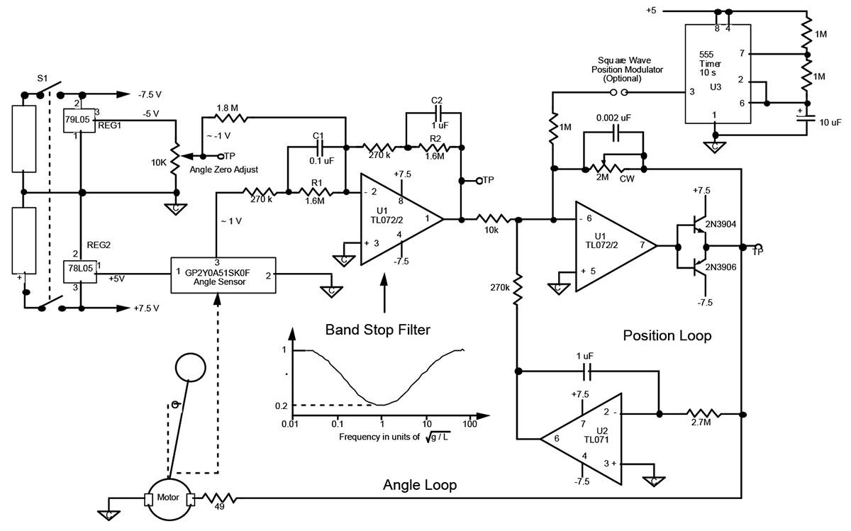
Figure 6. The schematic of the control system for stabilizing the inverted pendulum of Figure 2. Note that unlike Figure 5, the position signal is connected after the filter rather than before it. Since the position is a relatively slow signal, this makes little difference in the performance, but it saves one op-amp because the position signal at U2 pin 6 would have to be inverted if it fed in at U1 pin 2.

Component values are selected for a 0.5m pole (w_p = 4.4 rad/s). The dominant mass of the system is the battery pack (10 AAA cells).

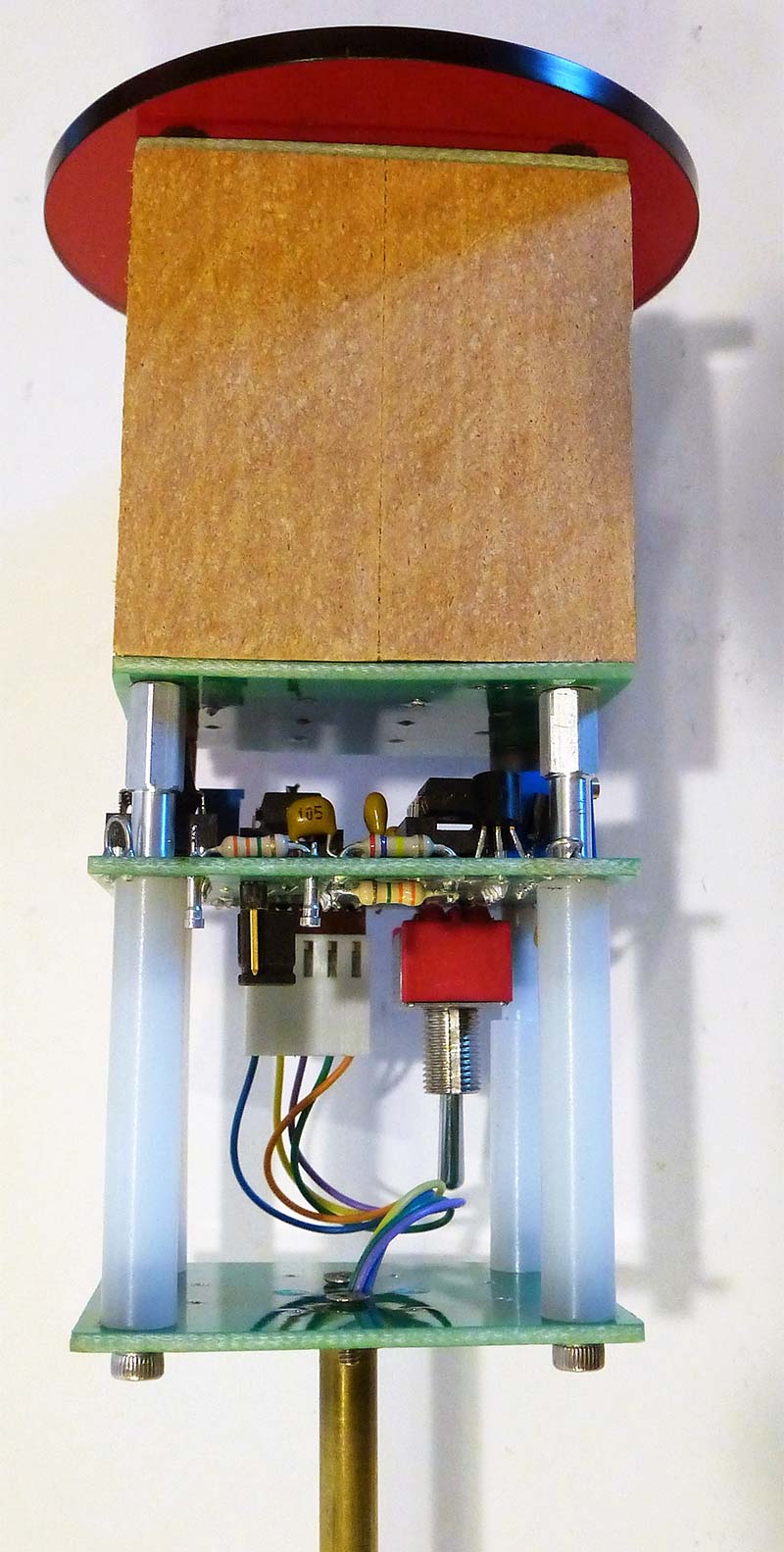
The battery pack and control circuitry are mounted at the top of the inverted pendulum

Except for the motor and wheels, all components including the batteries are placed at the top of the pole. This minimizes the mass of the cart and increases the maximum cart acceleration and recovery angle.

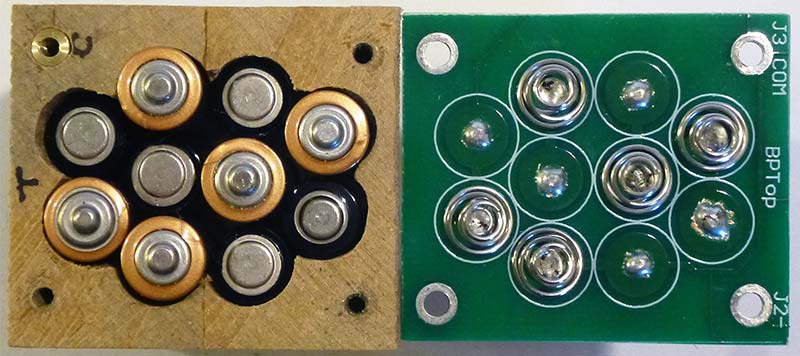
The AAA battery pack is shown with its top PCB removed. The 10 cells are wired to supply ±7.5V.

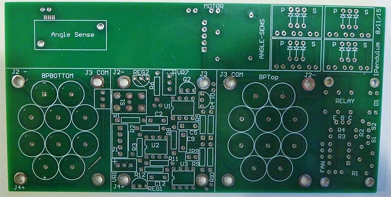
The four PCBs used in the test model are laid out on one board to reduce fab costs. They are the level sensor cantilever (top left); battery pack top (bottom left); control circuitry (bottom center); and battery pack bottom (bottom right). Additional circuits on the right side are unrelated to the inverted pendulum project.

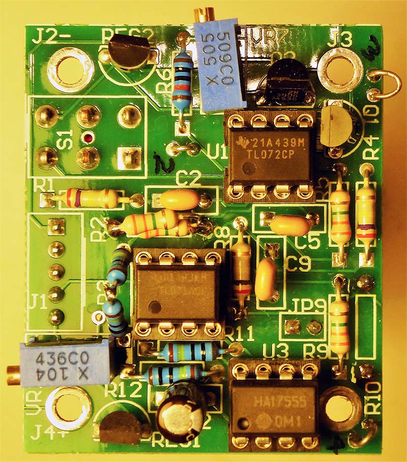
All of the control circuitry fits on this 1.9 x 2.1 inch PCB.

The motor is a typical small DC motor with a 40:1 gear-down ratio.

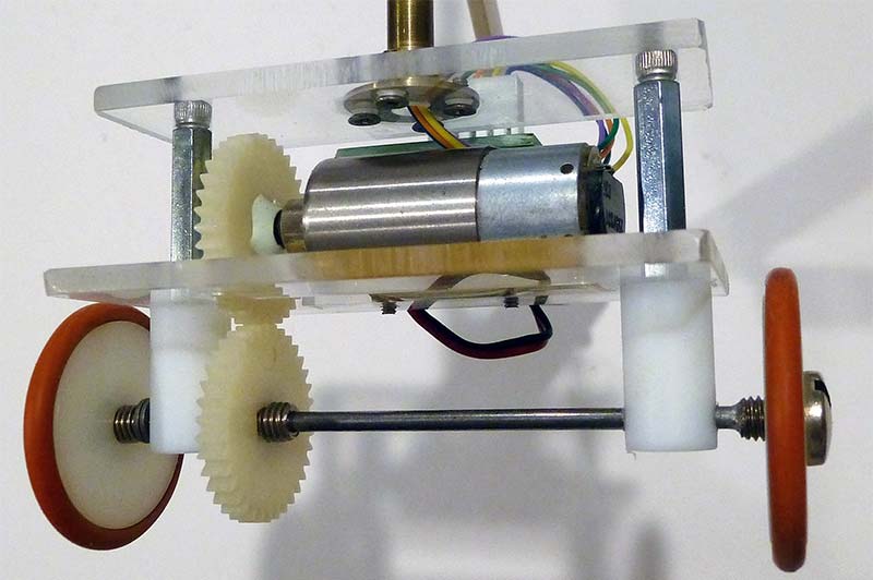
The 40:1 gearhead motor and drive wheels. Rubber O-rings on the wheels provide the required traction.

Plus and minus 5V regulators are used for the angle offset adjustment and to power the angle sensor. This makes the system insensitive to changing supply voltage as the batteries run down. The 49 ohm resistor in series with the motor tends to make it respond with torque vs. voltage rather than speed vs. voltage.

The position control has two inverting amplifiers in a loop that — by itself — is completely unstable. Without the rest of the system, the position loop will run away to saturation in about five seconds.

The band suppression filter can be intuitively explained as follows: At very low frequencies, C1 and C2 can be ignored. The input and feedback resistors are both 0.27 +1.6 = 1.8 MW, so the gain is 1. As the frequency rises, C2 (the larger capacitor) will begin to short out R2, reducing the feedback impedance causing the gain to drop.

As frequency continues to increase, C1 will begin shorting out R1, reducing the input impedance causing the gain to rise. At high frequencies, R1 and R2 are both shorted out by C1 and C2, so the gain comes back to 1.

Component values are chosen to put the low point at w_p = 4.4 rad/s. The 555 timer at the upper left is an optional position control that causes the command position to move left and right about 20 cm at 10 second intervals.

The realization of the stabilization algorithm described here has no accelerometers, no gyros, no bits, no code, and no processor. It’s a purely analog solution with just three op-amps and a few resistors and capacitors.

It illustrates the concepts of stabilization of the inverted pendulum without wading through the math and all of the many lines of code to be found in a microprocessor solution.

Over the years, I have built four versions of the stabilized inverted pendulum, from the 60 pound vacuum tube version of 1965 to the two-wheel 12 ounce version of Figure 2 — all using the same math, but each taking advantage of improved technology to produce a simpler and lower cost design.

If this problem sounds like fun, harvest a motor and some gears from a junked CD player and give it a try.

Stabilizing an inverted pendulum is a favorite and much discussed control theory problem for roboticists. The basic idea is illustrated in Figures 1 and 2. Simply put, the problem is to drive the robot base forward or backward in such a manner as to prevent the inverted pendulum design from falling over.

As you can now see, the math and science behind this task is not so bad after all. SV