Teaching a Robot to Play Catch With Minimal Mathematics

» Skip to the Extras

We wrote an article that discussed an unconventional approach to experimenting with machine intelligence. The comments we received on the article typically asked if the principles of such an approach could be applied to more complicated situations than the line following example used in that article. This article tries to address those queries by examining an alternative method for teaching a robot to predict the flight of a ball so it can be caught or batted back into the air.

Very few hobbyists would even consider building a robot that can catch a ball, not just because of the mechanical complexities of building such a robot but also because of the mathematics normally associated with such a task.

A typical mathematical approach to such a project would be to observe the ball long enough to develop an equation describing its path and then use that equation to predict where the ball will land. The robot could then move to that point and wait for the ball to arrive.

Surely, there is an easier way to solve this problem. After all, even a relatively young child can figure out how to catch a ball — and they certainly are not constructing complex equations to achieve their goal.

In our article on “Experimenting with Machine Intelligence” mentioned above, we suggested that robots can learn to solve problems by simply trying various actions and evaluating how well those actions help achieve the desired goal. Here, we will show that a robot using this simplified approach can learn to track the movement of a ball and predict where it will land without using complex mathematics.

In order to keep the project simple enough to be covered in a short magazine article, we will utilize a two-dimensional simulation to demonstrate the workability of our methodology.

The Input Data

In order to ensure that the principles explored with our simulation will apply to real world situations, the input data for our algorithm must be the same as what a real robot might use in a similar situation. Any ball-playing robot would have to use some form of vision system to determine the coordinates of the ball at various positions throughout the flight.

A real robot might do this with multiple cameras, but our simulation can extract this information from the simulation's animation parameters.

As mentioned earlier, these coordinates normally could be used to construct an equation describing the ball's flight path. Instead of creating an equation, though, our algorithm will only use this information to determine the ball's height and its horizontal speed.

Our approach requires far less mathematics since these two parameters are easily obtained with simple arithmetic (the height is the current y coordinate and speed is the difference between the last two x coordinates).

When we discussed this approach with math and engineering professors, they often said these two pieces of information would not be enough to reliably predict where the ball would land. They argued that the differences in the y coordinate would also have to be examined in order to determine if the ball was currently rising or falling.

It was also debated that more than two sets of coordinates would have to be analyzed as a unit in order to extract acceleration data (implying that velocity data alone would not be enough).

In general, we certainly agree with this assessment, if the robot were to make only one prediction. For our algorithm, though, the robot will constantly update its prediction of where the ball will land. Early predictions do not have to be precise because their major purpose is to start the robot moving toward the expected destination.

This early movement ensures that the robot will be close enough to the ball's impact position that only small movements will be needed (late in the ball's flight) to fine-tune the interception of the ball. If you watch baseball outfielders (especially those that are young or inexperienced), you will see this is exactly what they do.

When the ball is first hit, they make a quick assessment as to whether the ball will be short or long, and start moving in an appropriate direction. As the ball approaches them, they constantly adjust their movement to ensure they are properly positioned to make the catch.

Our simulation will allow the user to employ a sling-shot to initially launch the ball at various angles and speeds. The mouse is used to pull the ball back as shown in Figure 1.

FIGURE 1.

The distance pulled back controls the speed, and the pull-back angle controls the trajectory much like the program, Angry Birds. The robot (shown on the right side of the figure) will move left and right trying to make the ball bounce off the platform mounted above it.

After the ball bounces off the robot (or the ground if the robot did not make its way to the ball in time), the robot will again try to move to the new impact position. This action is very similar to a child trying to keep a balloon afloat by constantly moving to the balloon's new position and batting it back into the air.

The Algorithm

As promised earlier, the robot will use minimal mathematics to predict where the ball will land. Instead of trying to predict the actual flight of the ball, our robot will simply assume that the distance the ball will travel will be proportional to the ball's current horizontal velocity and its altitude as depicted by the expression:

Distance = k * HorzVelocity * Height

The constant k in the expression is a fudge-factor that tries to correlate the relationship between the distance traveled and other two variables. There are many factors that influence the value of k — some of which are the units of time and distance, as well as the force of gravity being used in the simulation.

Keep in mind, though, that this simple expression provides only a very rough guess of the value of how far the ball will travel — especially early in the ball's flight path — because it does not consider factors such as the ball's current acceleration or even if the ball is rising or falling.

As the ball approaches impact, the predictions made with this expression are much more accurate. This led us to believe there could be some value for k that would let the robot perform much like a baseball outfielder. Furthermore, we felt it made sense to let the robot learn to catch the ball on its own by letting it self-modify the value of k based on the accuracy of its predictions.

If the value of k is too large, the predicted distance will be too long. This will cause the robot to move past the actual impact point as shown in Figure 2.

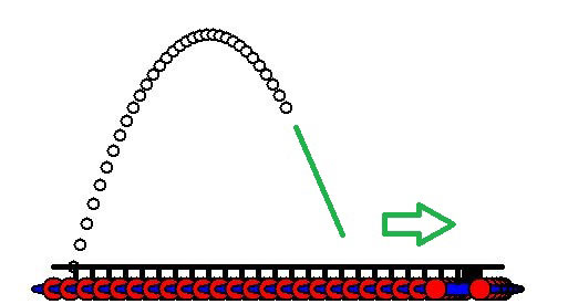
FIGURE 2.

This figure was created by modifying the simulation program so that it does not erase the old positions of the ball and robot during the animation process. In this case, the ball has just been batted into the air and the robot is moving to the right to intercept it. Since the prediction is too large, the robot moves well past where the ball will actually land (as depicted by the green line).

Notice also in this example, that the robot has already realized its error and has started moving back to the left. When the predicted distance-to-impact is too long — as it was here — the robot should decrease the value of k so that future predictions will have a better chance of being correct.

If the value of k is too small, then the predicted distance will be too short as shown in Figure 3.

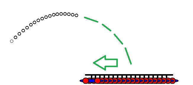
FIGURE 3.

In this case, the ball is moving toward the robot but the predicted travel distance is far too short, making the robot move much too far to the left. When this happens, the robot should increase the value of k. If the robot continually increases or decreases the value of k — based on the correctness of its prediction — it will eventually find a value that works as shown in Figure 4.

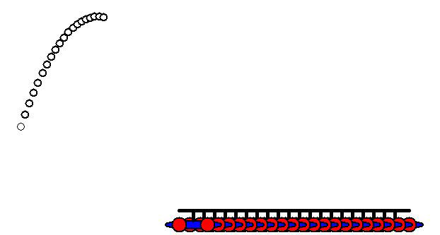
FIGURE 4.

As you can see, after the robot has established an appropriate value for k it will move to a position very close to where the ball will actually land.

Figure 5 shows the continuation of the ball's flight from Figure 4.

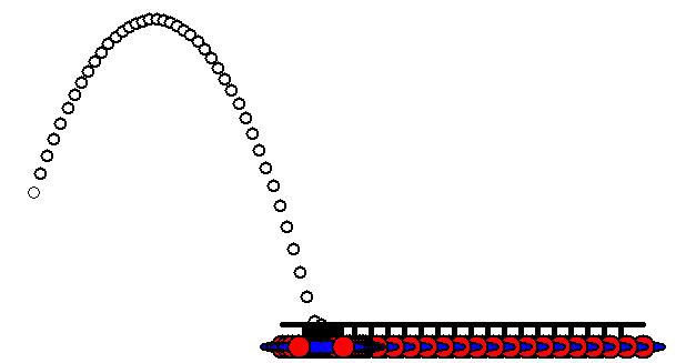
FIGURE 5.

Notice the robot did move slightly to the right in order to center itself at the impact point. Such corrections are more precise because the predictions of our algorithm become more accurate as the ball approaches impact.

It's important to realize that there is no one correct value for the constant k. The value is contingent on many factors, including the ball's current acceleration and its current angle of ascent and descent — all things our algorithm does not consider. Our simulations shows, however, that once the robot finds a reasonable value for k, it will work for nearly any reasonable situation.

We demonstrate this by making the simulated robot occasionally bat the ball back into the air with a random angle and velocity. This also ensures that the robot learns to handle a variety of trajectories and ball heights.

Furthermore, our robot never assumes that the value for k is correct. It continually modifies k based on how well the last prediction matched the actual impact position. Our simulation displays the current value of k at the top of the screen to help you see what is happening.

Determining Success or Failure

Implementing this algorithm requires the robot to evaluate the accuracy of its predictions. There are many ways to determine this. The robot could, for example, create a table of every prediction made during the ball’s flight and average them together to get a number to compare to where the ball eventually landed.

We actually tried that approach — along with several other ideas — and determined that almost anything reasonable will work. In fact, we even tried different expressions for predicting the distance. In the end, we found that any reasonable expression and any reasonable evaluation methodology seemed to produce a satisfactory solution.

Don't gloss over this point lightly. It suggests that robotic algorithms may not need the precise data or intricate equations that are often used to perform complex tasks. Remember also, that this simplified approach works because the robot continually adjusts its behavior rather than trying to predict everything in advance.

The final version of our program uses a very simple way of determining the accuracy of the predictions made. Our robot simply remembers the prediction impact position shortly after the ball starts to descend. This value is later compared to the actual impact point. If the ball traveled farther than expected, k is decreased by 5% of its value.

If the ball traveled less than predicted, the value of k is increased by 5%. Since this methodology only alters k by a slight amount, it can take awhile for the robot to become adept if the starting value of k is unreasonable. If the initial value of k is even somewhat appropriate, the robot will perform well after a very short learning period.

The fully commented source code for the program is less than 160 lines, and most of that is used for the simulation itself. Since the code is too long to list here, you can get it from the downloads or from the IN THE NEWS tab at www.RobotBASIC.org. Don't forget to download your free copy of RobotBASIC while you are there.

The comments in the code should make it easy for you to examine the algorithm and modify it to test various ideas of your own. For example, you could make the robot learn much faster by altering the value of k by a much larger percentage when the prediction is significantly different from the actual impact point.

In conclusion, we have demonstrated that the algorithms used to control a robot's behavior do not have to be as complicated as you might first assume.

The next time you are ready to program your robot to perform a complicated task, consider using a simulation to evaluate some simpler alternatives.

We think you will be surprised at how well your robot can perform when you let it play even a small role in deciding how and what it should do to accomplish its goals. SV