Alternative Computing Models: Part 3 — Electronic Analog Computing

» Skip to the Extras

In this third article of alternative computing models, we’ll explore electronic analog computing. As you’ll see from building your own analog computer with only a handful of inexpensive parts, analog computing can be as simple as automating a circular slide rule.

History

Although mechanical analog computing dates back to at least 2,000 years and the Greek Antikythera mechanism, modern analog computing dates back to the turn of the 20th century and the development of military targeting systems. These early systems — called fire control systems — were employed by the Royal Navy and later by the Imperial Russian Navy in World War I.

Similarly, thanks to military funding for R&D, the first fully electronic analog computing dates to 1942 and World War II. These embedded or onboard computers were used as guidance systems for German V-2 rockets.

After the war, development of analog computers accelerated in domestic, government, and military markets. For example, in 1952, RCA developed a room-sized computer consisting of 4,000 vacuum tubes.

The early electronic analog computers were fast — even by today’s standards — when applied to modeling and simulation of systems. By the early 1960s, affordable electronic analog computing was available to the enthusiast market through familiar brands such HeathKit, Edmund Scientific, and General Electric.

I purchased my first analog computer (a kit from Edmund Scientific) in 1965.

I have to admit that for the price (around $50) I was initially disappointed when I received the kit in the mail. It consisted of a cardboard box, three potentiometers, a switch, a small galvanometer, a double A battery holder, a few feet of 22 Ga wire, and three printed discs.

Despite the flimsy construction, the completed kit worked as advertised. I could multiply two numbers and read the product, add logarithms, and compute basic trig functions. The answers were accurate to within about 5% — almost as good as what I could achieve with my Picket slide rule.

My first experience with a “real” analog computer came several years later in the bilge of an old tugboat. I had to repair the automatic navigation system — a fully operational analog computer system based on a tube-type amplifier, a magnetic compass sensor, a rudder control motor, and a speed sensor.

Today, ships, boats, and just about every vehicle out there uses much more accurate GPS digital control systems that rely on satellites for position and speed information.

The Circuit

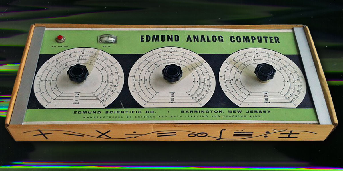
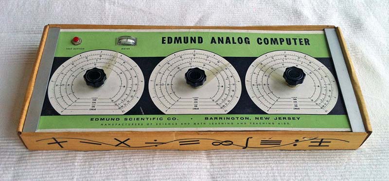
To understand basic electronic analog computing, we’re going to recreate a modified version of my Edmund Scientific computer kit from 60 years ago. Figure 1 shows the user interface which consists of three potentiometers and a galvanometer that I repurposed from a 1960’s circuit

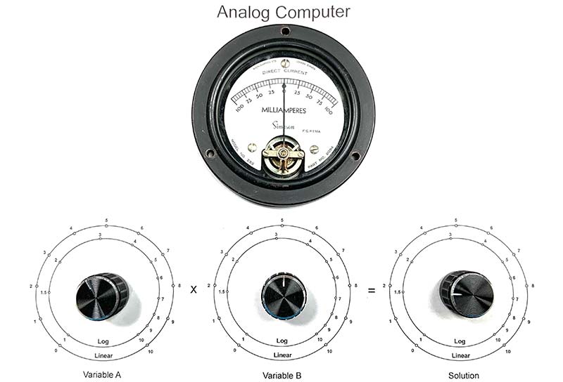
Figure 1. Electronic analog computer configured for multiplication and log mathematics.

Figure 2 shows the schematic for the computer.

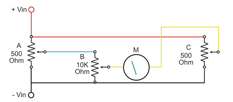
Figure 2. Schematic for the analog computer.

In my case, power (about a volt at a few milliamps) is supplied by a bench supply with a current limiter (Figure 3).

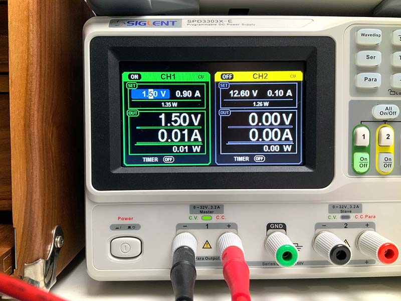
Figure 3. Power supplied by a bench supply.

Alternatively, you can use a single AA battery and a switch to cut off power when the computer is not in use.

As you can see, the circuit is about as simple as it gets. A pair of 500 ohm linear potentiometers, a 10K ohm linear potentiometer, and a galvanometer are used to create a voltage divider circuit.

Let’s say we’re using the computer as a multiplication engine. When the position of potentiometer C is equal to the product of potentiometer position A and potentiometer position B, then the voltages on the wiper arms of potentiometers B and C are equal.

That is, the galvanometer reads zero. When there is a voltage difference between the wiper arms, the galvanometer reads positive or negative.

The actual value of Vin isn’t that important. The voltage used should be sufficient to show meter activity but not so great as to burn out a potentiometer if the wiper arm is at the extreme clockwise / counterclockwise position. About a volt works for me. A current-limited supply ensures that I won’t burn out a potentiometer.

The Build

Keeping true to the kit that inspired this computer, it’s based on a sheet of cardboard and front panel printed with my laser printer. The hardest part of the build is creating the three identical dials corresponding to variables A and B and the product C.

Figure 4 shows a close-up of dial B.

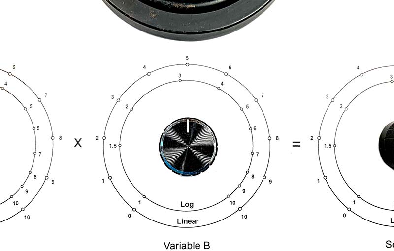
Figure 4. Dial B, which is identical to the other two dials.

Note that the knob has a simple line to indicate rotational position. Feel free to substitute knobs with long clear plastic points or some other indicator.

Figure 5 shows the back of the computer.

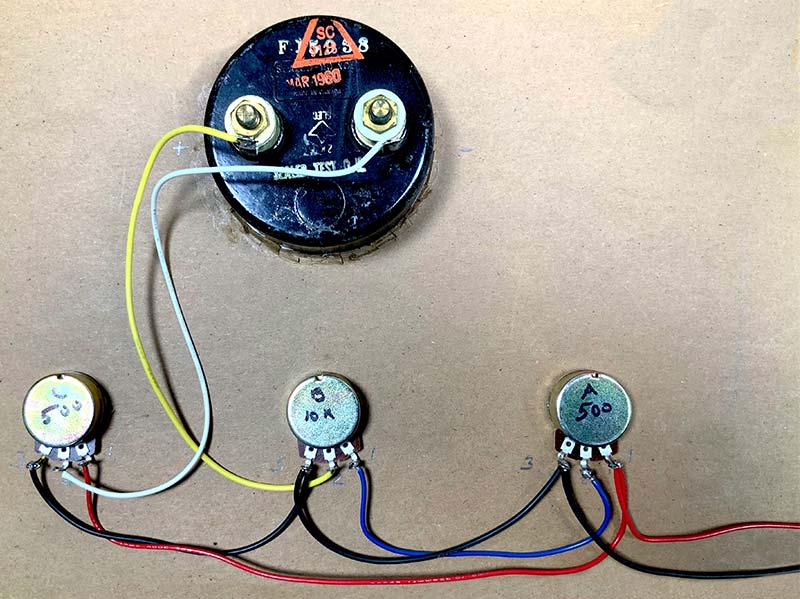
Figure 5. Computer wiring.

As you can see, wiring follows the schematic down to the color of the wires (with the exception of the white wire).

The three potentiometers are mounted through the cardboard and secured with nuts; the galvanometer is a press fit. The black and red wires on the bottom right lead to the power supply.

I purchased the two 500 ohm at 0.25W and single 10K ohm at 0.25W potentiometers from Amazon. Each value is available as three units, with matching black aluminum knobs and all necessary mounting hardware for $11. So, total cost of the two sets of three potentiometers is $22.

The particular galvanometer used in my computer was a special purchase from eBay. I didn’t mind spending $18 for a period-correct meter. You should be able to find less expensive modern galvanometers on eBay.

Another alternative is to use your DMM to indicate the solution position of potentiometer C. Speaking from experience, you can avoid burning out the fuse in your DMM by measuring voltage instead of current flow.

Hands On

If you’ve followed this series — especially the last article on the slide rule — then operating this computer should be second nature. As back in Figure 1, when Variable A is set to 4 and Variable B is set to 0.5, then the product can be read as 2 on the far right.

Until you zero in on the 2 value for potentiometer C, the galvanometer will read as positive or negative as shown in Figure 6.

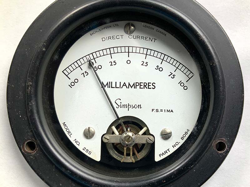
Figure 6. Galvanometer indicating the position of potentiometer C is incorrect.

As with a slide rule, you have to keep track of the decimal point. The same position of the knob on potentiometer C could be interpreted as 2, 20, 200, or 200,000.

You’ve probably noticed that I’ve added a log scale along with the linear scale. You can add other functions to the computer by adding value rings. In short, if you can perform a function on a slide rule — square root, cube root, trig — then you can do it with this computer.

Where to Go From Here

From the perspective of a better electronic analog computer, it’s easy to extend the design by adding discs or potentiometer position value markers that represent trigonometry or other math functions. I’ve included a PDF of the front panel as well as a 6” disc in the article downloads that you can use together with precision potentiometers to create a higher resolution version of the computer. You can also consider adding pointers to the knobs.

I tried to keep the design true to the original, using flimsy cardboard and a plain black and white interface. But consider a plastic enclosure and small meters as well as color-coded rings showing position values.

An easy and fun modification to this design is to forgo the meter and to insert a pair of headphones where the meter would go. Instead of a 1 VDC supply, feed the system with a tone from a signal generator or your MP3 player. A null in volume indicates that potentiometer C is at the solution position. You can also dig deeper into analog computing by moving from a steady state DC circuit to a pulsed circuit and adding capacitors to the mix.

Now you’re capable of differential equations with values set by adjusting the RC values. Given the proper mix of multiplier and specialized math modules, you can create complex, real time computational systems that rival modern desktop digital systems in terms of speed.

From the perspective of this series, I hope that you have at least entertained the thought that computers, robotics, and other computational systems are not limited to a digital paradigm.

Take a look at some of the modern hybrid analog-digital systems commercially available to handle problems that would be impractical for a digital-only approach. SV